The provided content outlines a comprehensive backtesting analysis of an SMA (Simple Moving Average) cross strategy applied to AMD (Advanced Micro Devices) stock data, with a focus on optimizing the strategy through long/short SMA length tuning to outperform Buy & Hold returns.
Abstract
The article delves into the application of vectorized backtesting to evaluate the performance of an SMA cross strategy for AMD stock from 2019 to 2024. It emphasizes the importance of hyperparameter optimization in machine learning, akin to finding the optimal SMA lengths for trading. The study iterates over 9,165 combinations of short and long SMA lengths to identify the most profitable strategy, ultimately pinpointing the optimal SMA lengths as 47 and 86. The analysis includes descriptive statistics of AMD's stock returns, the use of technical indicators such as EMA, RSI, and Bollinger Bands, and a comparison of the SMA strategy's performance against the Buy & Hold approach. The optimal SMA strategy is further validated through deployment via Backtesting 0.3.3, demonstrating its potential for superior returns and risk management.
Opinions
The author believes that AMD is a prime candidate for algorithmic trading strategies due to its strong performance metrics and growth in the semiconductor industry.
There is an opinion that automated optimization of trading strategies, specifically SMA cross strategies, can lead to better returns than passive investment strategies like Buy & Hold.
The article suggests that the use of vectorized backtesting is an efficient method for testing trading strategies across a wide range of parameters.
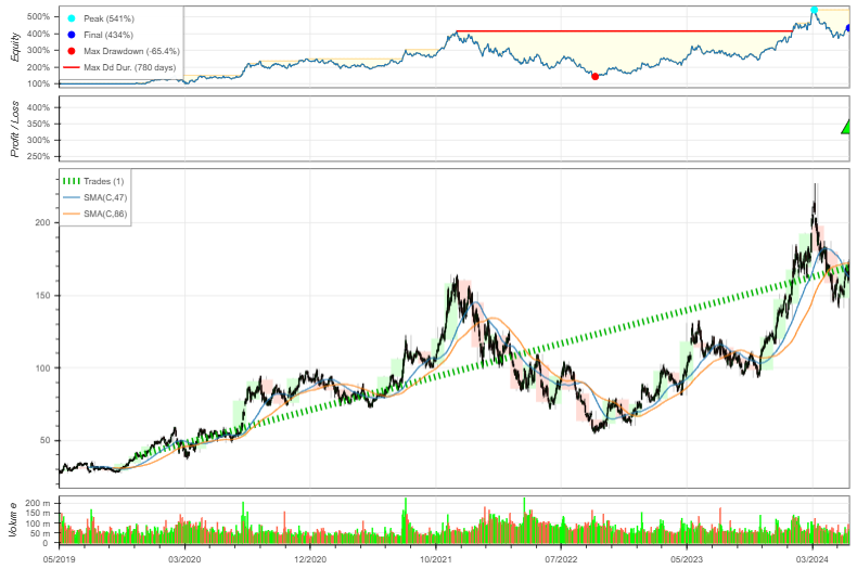
The author conveys that the optimal SMA strategy, once deployed, can yield significant returns, as evidenced by the backtesting results.
There is a cautious optimism regarding the use of backtesting, with a reminder that it should be complemented by other risk management strategies and a thorough understanding of market dynamics before live trading.
The article implies that technical indicators, when combined and properly tuned, can provide valuable insights for trading decisions.
Backtesting AMD Algo-Trading SMA Cross Strategy: Long/Short Auto Tuning vs Buy&Hold
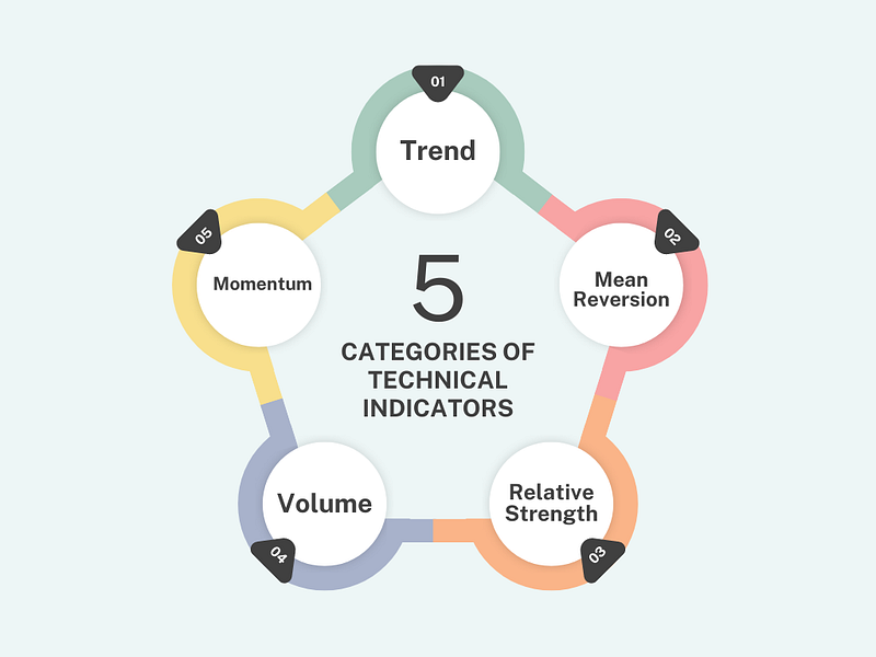
5 Main Categories of Technical Indicators
The present study aims at vectorized backtestingAMD algo-trading Simple Moving Average (SMA) cross strategy 2019–2024.
Here, the main focus is on long/short length auto tuning to maximize expected SMA strategy returns while outperforming the passive Buy&Hold returns.
As with hyperparameter optimization in ML, we will iterate over various combinations of SMA lengths to find the optimal (hyper) parameters that maximize the annual returns/risk ratio.
In a nutshell, this paper is about automated optimization of the SMA cross strategy under the umbrella of vectorized backtesting.
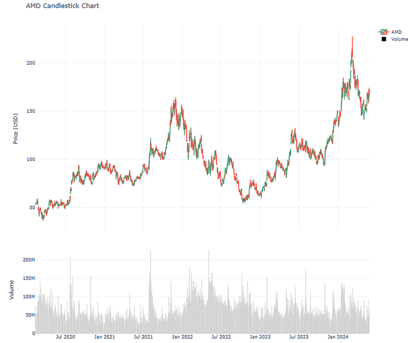
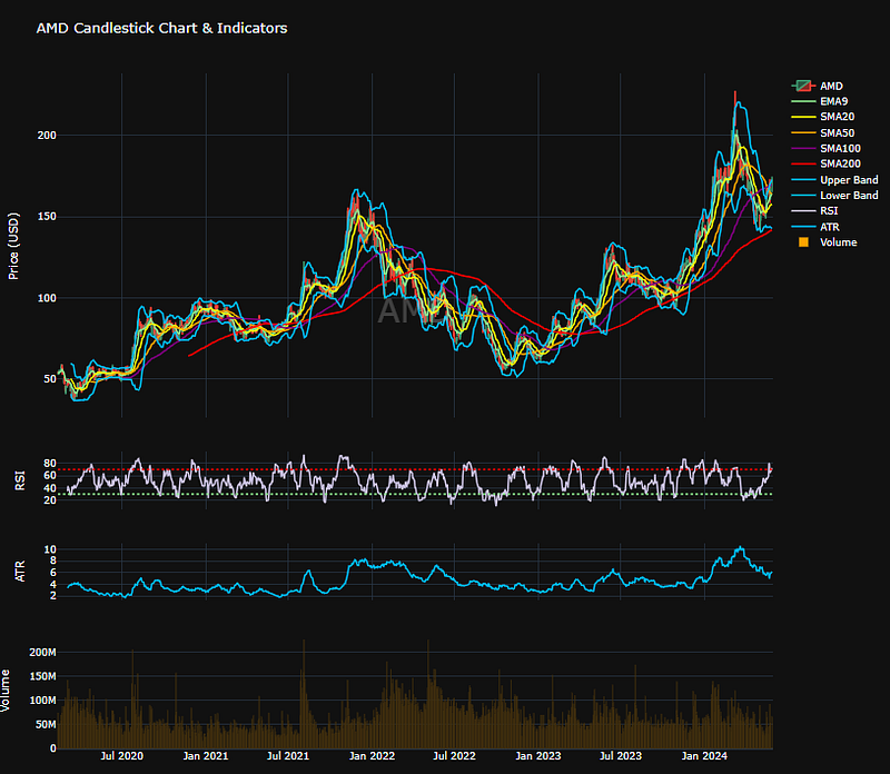
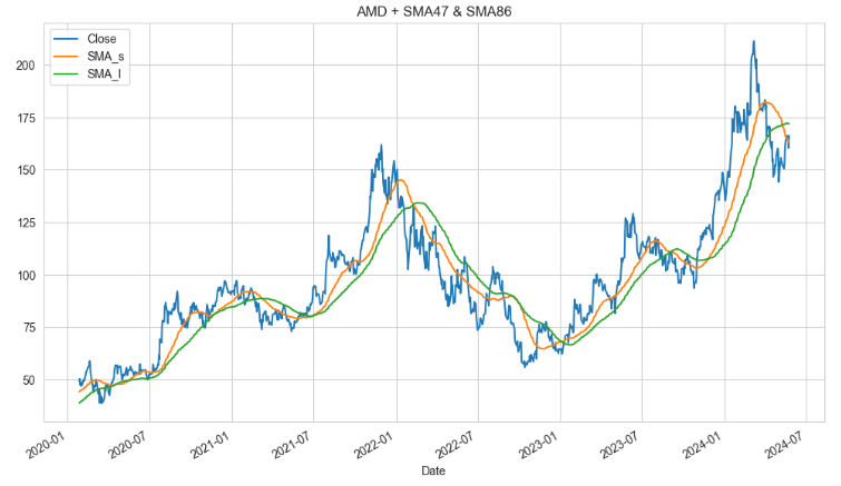
Plotting the Plotly Candlesticks with/without Indicators
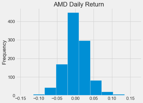
Descriptive statistics (kurtosis, skewness, std, etc.) of daily returns
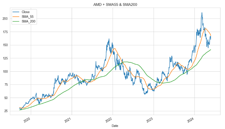
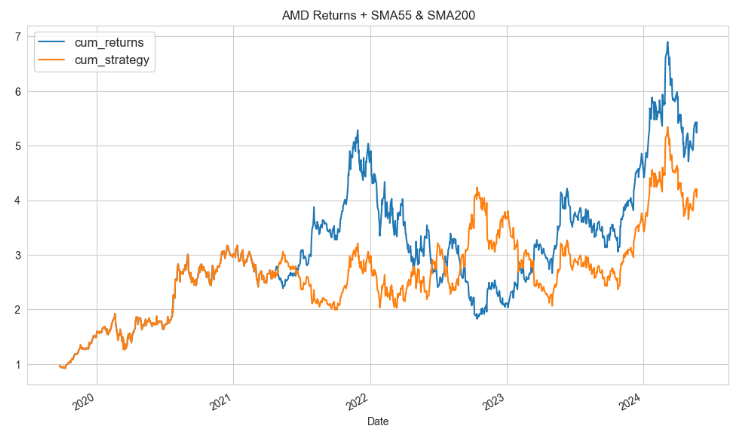
Examining the Default SMA 55/200 Cross Strategy
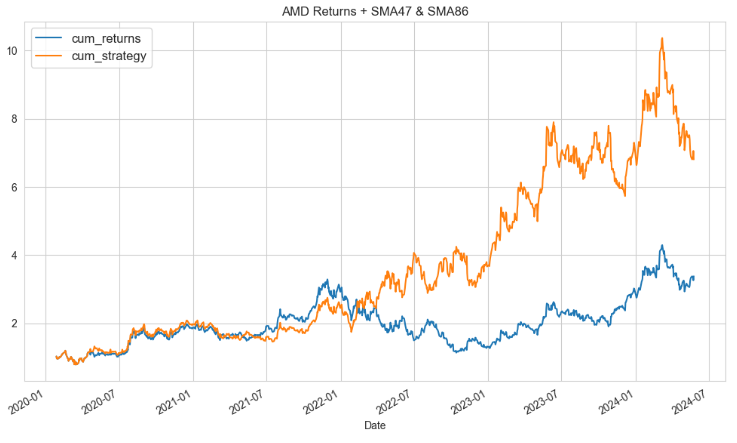
Finding the Optimal SMA (47/86) Cross Strategy by iterating over 9165 combinations of Short/Long lengths
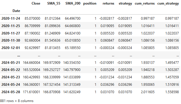
Defining position and calculating strategy returns
Comparing absolute performance and annual returns/risk: SMA strategy vs Buy&Hold
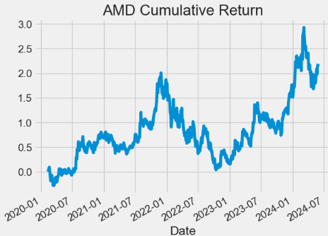
Calculating and visualizing cumulative returns of SMA vs benchmark
Optimal SMA Strategy Deployment via Backtesting 0.3.3
Introduction to the SMA Indicator
The SMA is an arithmetic moving average calculated by adding recent prices and then dividing that figure by the number of time periods in the calculation average.
The SMA is a trend indicator that smooths price movements to filter out the noise of an asset. Traders frequently use SMA to open/close trades through SMA crossovers, and to find supports and resistances in different time frames. These crossovers are generated by predefining two moving averages, a slow and a fast one. The slow SMA takes into account a larger amount of periods, then catching the general trend of the asset. And the fast SMA is calculated with fewer periods, reacting quicker to price movements.
During a bearish trend, when the fast SMA crosses the slow one upward, the trend is likely to have a reversal and the BUY signal. However, in a bullish trend and the fast SMA crosses the slow one downward, we will get the SELL signal.
Basic Setup & Input Stock Data
Setting the working directory YOURPATH
import os
os.chdir('YOURPATH')    # Set working directory
os. getcwd()
Importing the necessary libraries
import datetime
import pandas as pd
import numpy as np
import matplotlib.pyplot as plt
import seaborn as sns
import plotly.graph_objects as go
sns.set_style("whitegrid")
from itertools import product
import yfinance as yf
# ignore the warningsimport warnings
warnings.filterwarnings('ignore')
Reading the input historical stock data using get_data
#daily datadefget_data(pairs):
global df, symbol
NUM_DAYS = 2000# The number of days of historical data to retrieve#define start & dates
start = (datetime.date.today() - datetime.timedelta( NUM_DAYS ) )
end = datetime.datetime.today()
#pull data
df = yf.download(pairs, start=start)
return df
pair = "AMD"
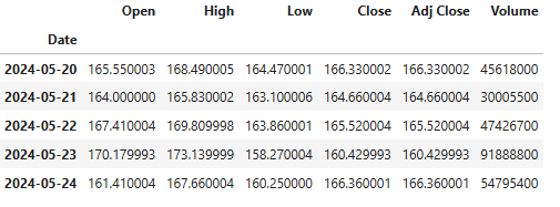
df = get_data(pair)
df.tail()
AMD historical stock data
Printing the descriptive summary statistics of Close price
Iterating through sma_short = and sma_long ranges [3,50] and [55,250], respectively, viz.
#range of sma
range_sma_short = range(3, 50, 1)
range_sma_long = range(55, 250, 1)
#combination of SMAs
smas = list(product(range_sma_short, range_sma_long))
smas
[(3, 55),
(3, 56),
(3, 57),
.........
(8, 76),
(8, 77),
(8, 78),
(8, 79),
...]
#iterate through sma combination and test strategy
abs_perform = []
for pro in smas:
abs_perform.append(sma_backtest(data, pro[0], pro[1]))
#get max performance value
np.max(abs_perform)
6.8029#get max value combination
best_comb = smas[np.argmax(abs_perform)]
best_comb
(47, 86)
Creating the summary performance DataFrame
#results to dataframe
results = pd.DataFrame(smas, columns = ["SMA_short", "SMA_long"])
results
SMA_short SMA_long
03551356235733584359... ... ...
9160492459161492469162492479163492489164492499165 rows × 2 columns
results["abs_performance"] = abs_perform
results
SMA_short SMA_long abs_performance
03551.8670613561.4994823571.2039233581.2571943591.34725... ... ... ...
9160492451.353109161492461.335309162492471.317889163492481.252689164492491.254489165 rows × 3 columns
#top 10 best performing combination
best = results.nlargest(10, "abs_performance")
best
SMA_short SMA_long abs_performance
861147866.80290900249876.441407489411346.39373841646866.23989841746876.139697487411326.035757681421315.987457488411335.975107682421325.961437294401345.96075#top 10 least performing combination
least = results.nsmallest(10, "abs_performance")
least
SMA_short SMA_long abs_performance
488628660.68864546931640.69114508229670.70002527530650.7137115932140.72108469027650.721773945590.73426412424840.74273527430640.74340507929640.75038
We have implemented and tested the automated backtesting procedure of applying the SMA trading strategy to historical AMD data to determine its efficacy and to optimize its performance. It is a way to test a strategy without risking real capital.
The idea is that a trading strategy that did well in the past will produce a better result in the future.
Our backtesting is associated with an automated trading system or a bot. This is a piece of software that does hands-off analysis and then executes trades. It can also set a stop-loss and a take-profit to properly manage risks.
The near-term project will involve vectorized backtesting of multiple trading indicators with (hyper) parameter optimization beyond the simple SMA strategy.
Backtesting trading strategies will also be used to test different strategies and determine which ones are more profitable.
Disclaimer: Backtesting should be used in conjunction with other risk management strategies, fundamental analysis, and a deep understanding of market dynamics before deploying capital in real-world trading.