Backtesting Hybrid CI & MACD Trading Strategies for NVIDIA

AI the future: How NVIDIA is changing the digital world

Featured image template via Canva.

In this post, we’ll take a closer look at backtesting NVIDIA (NASDAQ: NVDA) algo-trading strategies in Python that maximize the ROI/Risk ratio by combining Chopping Index (CHOP/CI) & MACD technical indicators, as explained here.
The CI indicates whether a choppy market exists. A choppy market refers to a period of market volatility where a trend is generally absent.
As a range-bound oscillator, the CI has values within the range [1,100]. The closer the value is to 100, the higher the sideways movement levels.
A CI value above MAX0=61.8 indicates a trending market, while a value below MIN0=38.2 indicates a choppy market.
In this study, we’ll set MIN=50 and MAX=MAX0 because the default value MIN0 leads to lower ROI for NVDA within the time frame of interest.
The Moving Average Convergence/Divergence (MACD) indicator is designed to help investors identify price trends, measure trend momentum, and identify market entry points for buying or selling.
MACD is best used with daily periods, where the traditional settings of 26/12/9 days is the default.
Why CI + MACD: While the MACD is effective in trend confirmation, the CI can quickly respond to immediate price fluctuations if the market is trading sideways.
Let’s get down to implementation details!

Reading Input Stock Data

Setting the working directory YOURPATH

import os
os.chdir('YOURPATH')    # Set working directory
os. getcwd()

Importing basic libraries and reading the 2Y NVDA historical data

import pandas as pd
import requests
import matplotlib.pyplot as plt
import numpy as np

plt.style.use('fivethirtyeight')
plt.rcParams['figure.figsize'] = (20, 10)

def get_historical_data(symbol, start_date):
    api_key = 'YOUR API KEY'
    api_url = f'https://api.twelvedata.com/time_series?symbol={symbol}&interval=1day&outputsize=5000&apikey={api_key}'
    raw_df = requests.get(api_url).json()
    df = pd.DataFrame(raw_df['values']).iloc[::-1].set_index('datetime').astype(float)
    df = df[df.index >= start_date]
    df.index = pd.to_datetime(df.index)
    return df

tsla = get_historical_data('NVDA', '2022-01-01')
tsla

           open      high      low       close     volume
datetime     
2022-01-03 298.14999 307.10999 297.85001 301.20999 39240296.0
2022-01-04 302.76999 304.67999 283.48999 292.89999 52715440.0
2022-01-05 289.48999 294.16000 275.32999 276.04001 49806388.0
2022-01-06 276.39999 284.37991 270.64999 281.78000 45418636.0
2022-01-07 281.41000 284.22000 270.57001 272.47000 40993852.0
... ... ... ... ... ...
2024-04-05 868.65997 884.81000 859.26001 880.08002 39885700.0
2024-04-08 887.00000 888.29999 867.32001 871.33002 28322000.0
2024-04-09 874.41998 876.34998 830.21997 853.53998 50354700.0
2024-04-10 839.26001 874.00000 837.09003 870.39001 43192900.0
2024-04-11 874.20001 907.39001 869.26001 906.15997 42969300.0
571 rows × 5 columns

CI Indicator

Calculating and plotting the CI 14 indicator

def get_ci(high, low, close, lookback):
    tr1 = pd.DataFrame(high - low).rename(columns = {0:'tr1'})
    tr2 = pd.DataFrame(abs(high - close.shift(1))).rename(columns = {0:'tr2'})
    tr3 = pd.DataFrame(abs(low - close.shift(1))).rename(columns = {0:'tr3'})
    frames = [tr1, tr2, tr3]
    tr = pd.concat(frames, axis = 1, join = 'inner').dropna().max(axis = 1)
    atr = tr.rolling(1).mean()
    highh = high.rolling(lookback).max()
    lowl = low.rolling(lookback).min()
    ci = 100 * np.log10((atr.rolling(lookback).sum()) / (highh - lowl)) / np.log10(lookback)
    return ci

tsla['ci_14'] = get_ci(tsla['high'], tsla['low'], tsla['close'], 14)
tsla = tsla.dropna()
tsla

ax1 = plt.subplot2grid((11,1,), (0,0), rowspan = 5, colspan = 1)
ax2 = plt.subplot2grid((11,1,), (6,0), rowspan = 4, colspan = 1)
ax1.plot(tsla['close'], linewidth = 2.5, color = '#2196f3')
ax1.set_title('NVDA CLOSING PRICES')
ax2.plot(tsla['ci_14'], linewidth = 2.5, color = '#fb8c00')
ax2.axhline(50, linestyle = '--', linewidth = 1.5, color = 'grey')
ax2.axhline(61.8, linestyle = '--', linewidth = 1.5, color = 'grey')
ax2.set_title('NVDA CHOPPINESS INDEX 14')
plt.show()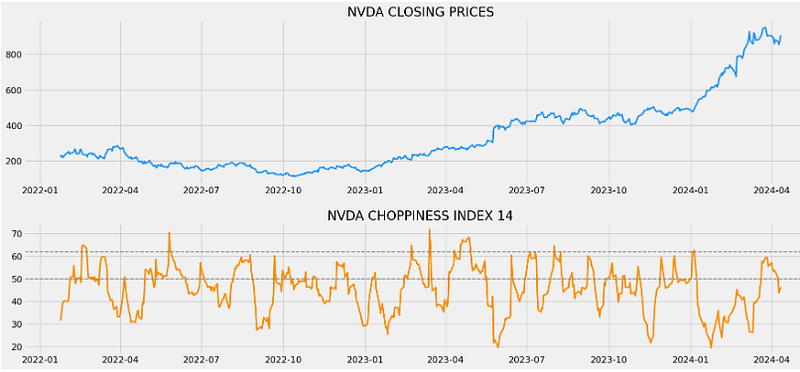

NVDA closing prices vs CI 14 with the signal range [50,61.8]

MACD Indicator

Calculating the MACD 26/12/9 indicator

def get_macd(price, slow, fast, smooth):
    exp1 = price.ewm(span = fast, adjust = False).mean()
    exp2 = price.ewm(span = slow, adjust = False).mean()
    macd = pd.DataFrame(exp1 - exp2).rename(columns = {'close':'macd'})
    signal = pd.DataFrame(macd.ewm(span = smooth, adjust = False).mean()).rename(columns = {'macd':'signal'})
    hist = pd.DataFrame(macd['macd'] - signal['signal']).rename(columns = {0:'hist'})
    frames =  [macd, signal, hist]
    df = pd.concat(frames, join = 'inner', axis = 1)
    return df

tsla_macd = get_macd(tsla['close'], 26, 12, 9)
tsla_macd.tail()
           macd      signal     hist
datetime   
2024-04-05 24.096374 37.124507 -13.028134
2024-04-08 20.667086 33.833023 -13.165937
2024-04-09 16.325652 30.331549 -14.005897
2024-04-10 14.082358 27.081711 -12.999353
2024-04-11 15.017752 24.668919 -9.65116

CI & MACD Trading Strategy

Implementing the hybrid CI & MACD trading strategy and plotting the resulting NVDA trading signals

par=50

# Implementing the CI & MACD trading strategy 

def implement_ci_macd_strategy(prices, data, ci):
    buy_price = []
    sell_price = []
    ci_macd_signal = []
    signal = 0
    
    for i in range(len(prices)):
        if data['macd'][i] > data['signal'][i] and ci[i] < par:
            if signal != 1:
                buy_price.append(prices[i])
                sell_price.append(np.nan)
                signal = 1
                ci_macd_signal.append(signal)
            else:
                buy_price.append(np.nan)
                sell_price.append(np.nan)
                ci_macd_signal.append(0)
        elif data['macd'][i] < data['signal'][i] and ci[i] < par:
            if signal != -1:
                buy_price.append(np.nan)
                sell_price.append(prices[i])
                signal = -1
                ci_macd_signal.append(signal)
            else:
                buy_price.append(np.nan)
                sell_price.append(np.nan)
                ci_macd_signal.append(0)
        else:
            buy_price.append(np.nan)
            sell_price.append(np.nan)
            ci_macd_signal.append(0)
    
    return buy_price, sell_price, ci_macd_signal

#Plotting CI & MACD trading signals

buy_price, sell_price, ci_macd_signal = implement_ci_macd_strategy(tsla['close'], tsla_macd, tsla['ci_14'])

ax1 = plt.subplot2grid((19,1,), (0,0), rowspan = 5, colspan = 1)
ax2 = plt.subplot2grid((19,1), (7,0), rowspan = 5, colspan = 1)
ax3 = plt.subplot2grid((19,1), (14,0), rowspan = 5, colspan = 1)
ax1.plot(tsla['close'], linewidth = 2.5, color = '#2196f3')
ax1.plot(tsla.index, buy_price, marker = '^', color = 'green', markersize = 12, label = 'BUY SIGNAL', linewidth = 0)
ax1.plot(tsla.index, sell_price, marker = 'v', color = 'r', markersize = 12, label = 'SELL SIGNAL', linewidth = 0)
ax1.legend()
ax1.set_title('NVDA TRADING SIGNALS')
ax2.plot(tsla['ci_14'], linewidth = 2.5, color = '#fb8c00')
ax2.axhline(50, linestyle = '--', linewidth = 1.5, color = 'grey')
ax2.axhline(61.8, linestyle = '--', linewidth = 1.5, color = 'grey')
ax2.set_title('NVDA CHOPPINESS INDEX 14')
ax3.plot(tsla_macd['macd'], color = 'grey', linewidth = 1.5, label = 'MACD')
ax3.plot(tsla_macd['signal'], color = 'skyblue', linewidth = 1.5, label = 'SIGNAL')
for i in range(len(tsla_macd)):
    if str(tsla_macd['hist'][i])[0] == '-':
        ax3.bar(tsla_macd.index[i], tsla_macd['hist'][i], color = '#ef5350')
    else:
        ax3.bar(tsla_macd.index[i], tsla_macd['hist'][i], color = '#26a69a')
ax3.legend()
ax3.set_title('NVDA MACD 26,12,9')
plt.show()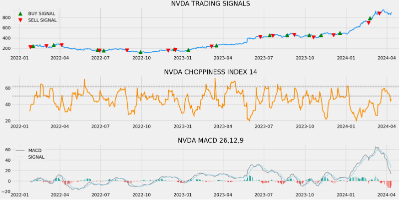

NVDA trading signals, CI 14, and MACD 26/12/9

Daily & Cumulative Returns

Formulating the NVDA stock trading position and calculating the daily/cumulative returns since 2022–01–01

osition = []
for i in range(len(ci_macd_signal)):
    if ci_macd_signal[i] > 1:
        position.append(0)
    else:
        position.append(1)
        
for i in range(len(tsla['close'])):
    if ci_macd_signal[i] == 1:
        position[i] = 1
    elif ci_macd_signal[i] == -1:
        position[i] = 0
    else:
        position[i] = position[i-1]
        
ci = tsla['ci_14']
close_price = tsla['close']
ci_macd_signal = pd.DataFrame(ci_macd_signal).rename(columns = {0:'ci_macd_signal'}).set_index(tsla.index)
position = pd.DataFrame(position).rename(columns = {0:'ci_macd_position'}).set_index(tsla.index)

frames = [close_price, ci, ci_macd_signal, position]
strategy = pd.concat(frames, join = 'inner', axis = 1)

strategy.head()

rets = tsla.close.pct_change()[1:]
strat_rets = strategy.ci_macd_position[1:] * rets

plt.title('Daily Returns')
rets.plot(color = 'blue', alpha = 0.3, linewidth = 7)
strat_rets.plot(color = 'r', linewidth = 1)
plt.show()

rets_cum = (1 + rets).cumprod() - 1 
strat_cum = (1 + strat_rets).cumprod() - 1

plt.title('Cumulative Returns')
rets_cum.plot(color = 'blue', alpha = 0.3, linewidth = 7)
strat_cum.plot(color = 'r', linewidth = 2)
plt.show()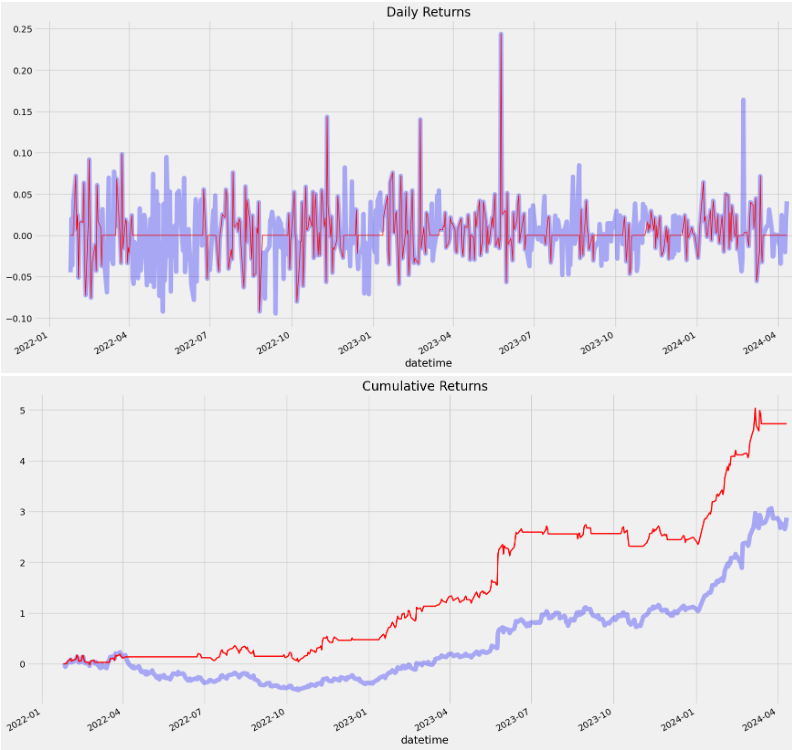

NVDA daily returns vs cumulative returns: buy-and-hold (blue) vs CI & MACD strategy (red)

Backtesting ROI

Calculating the profit gained from the CI-MACD strategy by investing $10k in NVDA

from termcolor import colored as cl 

fb_ret = pd.DataFrame(np.diff(tsla['close'])).rename(columns = {0:'returns'})
cci_strategy_ret = []

for i in range(len(fb_ret)):
    returns = fb_ret['returns'][i]*strategy['ci_macd_position'][i]
    cci_strategy_ret.append(returns)
    
cci_strategy_ret_df = pd.DataFrame(cci_strategy_ret).rename(columns = {0:'ci_macd_returns'})
investment_value = 10000
number_of_stocks = np.floor(investment_value/tsla['close'][-1])
cci_investment_ret = []

for i in range(len(cci_strategy_ret_df['ci_macd_returns'])):
    returns = number_of_stocks*cci_strategy_ret_df['ci_macd_returns'][i]
    cci_investment_ret.append(returns)

cci_investment_ret_df = pd.DataFrame(cci_investment_ret).rename(columns = {0:'investment_returns'})
total_investment_ret = round(sum(cci_investment_ret_df['investment_returns']), 2)
profit_percentage = round((total_investment_ret/investment_value)*100, 2)
print(cl('Profit gained from the CI-MACD strategy by investing $10k in NVDA : {}'.format(total_investment_ret), attrs = ['bold']))
print(cl('Profit percentage of the CI-MACD strategy : {}%'.format(profit_percentage), attrs = ['bold']))

Profit gained from the CI-MACD strategy by investing $10k in NVDA : 4908.31
Profit percentage of the CI-MACD strategy : 49.08%

SPY ETF Benchmark

Considering the SPY ETF benchmark

# SPY ETF COMPARISON


def get_benchmark(start_date, investment_value):
    spy = get_historical_data('SPY', start_date)['close']
    benchmark = pd.DataFrame(np.diff(spy)).rename(columns = {0:'benchmark_returns'})
    
    investment_value = investment_value
    number_of_stocks = np.floor(investment_value/spy[0])
    benchmark_investment_ret = []
    
    for i in range(len(benchmark['benchmark_returns'])):
        returns = number_of_stocks*benchmark['benchmark_returns'][i]
        benchmark_investment_ret.append(returns)

    benchmark_investment_ret_df = pd.DataFrame(benchmark_investment_ret).rename(columns = {0:'investment_returns'})
    return benchmark_investment_ret_df

benchmark = get_benchmark('2022-01-01', 10000)
investment_value = 10000
total_benchmark_investment_ret = round(sum(benchmark['investment_returns']), 2)
benchmark_profit_percentage = np.floor((total_benchmark_investment_ret/investment_value)*100)
print(cl('Benchmark profit by investing $10k : {}'.format(total_benchmark_investment_ret), attrs = ['bold']))
print(cl('Benchmark Profit percentage : {}%'.format(benchmark_profit_percentage), attrs = ['bold']))
print(cl('CI-MACD Strategy profit is {}% higher than the Benchmark Profit'.format(profit_percentage - benchmark_profit_percentage), attrs = ['bold']))

Benchmark profit by investing $10k : 805.8
Benchmark Profit percentage : 8.0%
CI-MACD Strategy profit is 41.08% higher than the Benchmark Profit

Conclusions

We have shown that the hybrid CI & MACD algo-trading strategy is a valuable tool in analyzing market trends, sideways movements and making informed trading decisions. Specifically, CI helps distinguish sideways movements from trending market activity, while it’s also used to evaluate an asset’s volatility.
This article describes the purpose, calculation, and application of this efficient strategy.
2Y backtesting results: ROI of the strategy is 49.08%.
2Y SPY ETF benchmark: the strategy ROI is 41.08% higher than the benchmark.
Future work: predicting NVDA stock price using ML/AI and statistical modeling approaches.