BTC Price Prediction using FB Prophet

Image design template courtesy of Canva.

In this article we are going to discuss the BTC price prediction using the FB Prophet algorithm in Python.
Utilizing historical BTC-USD data, the project employs this statistical modeling library to predict future BTC prices, contributing to informed decision-making in cryptocurrency markets.
Predicting the BTC price accurately is a difficult task due to its high volatility. One of the major problems with many price predictions about BTC is that they lack sufficient analytical support to back up their claims.
Where Prophet shines: It appears that by combining automatic forecasting with analyst-in-the-loop forecasts for special cases, it is possible to cover a wide variety of business use-cases.
At its core, the Prophet procedure is a regression model with four main components: a piecewise linear or logistic growth curve trend; a yearly seasonal component modeled using Fourier series; a weekly seasonal component using dummy variables; a user-provided list of important holidays.
Let’s delve into details.

Basic Imports, Installations & Setups

Installing and activating the slim Miniconda environment from cmd

conda activate my-conda-env

To deactivate this environment on Windows, run

conda deactivate

Launching the Jupyter Notebook

jupyter notebook

Creating a new project in the Notebook and selecting Python-3.
Setting a working directory YOURPATH

import os
os.chdir('YOURPATH')    # Set working directory
os. getcwd()

Importing and installing the following Python libraries

!pip install plotly, statsmodels, termcolor, math, requests, prophet, itertools
import pandas as pd
import plotly.express as px
import requests
import numpy as np
import matplotlib.pyplot as plt
from math import floor
from termcolor import colored as cl
from statsmodels.base.transform import BoxCox
from prophet import Prophet

plt.rcParams['figure.figsize'] = (20, 10)
plt.style.use('fivethirtyeight')

Reading & Plotting Input Data

Reading the Bitcoin USD (BTC-USD) stock data 2021/01–2023/09

def get_crypto_price(symbol, exchange, start_date = None):
    api_key = 'YOUR_API_KEY'
    api_url = f'https://www.alphavantage.co/query?function=DIGITAL_CURRENCY_DAILY&symbol={symbol}&market={exchange}&apikey={api_key}'
    raw_df = requests.get(api_url).json()
    df = pd.DataFrame(raw_df['Time Series (Digital Currency Daily)']).T
    df = df.rename(columns = {'1a. open (USD)': 'Open', '2a. high (USD)': 'High', '3a. low (USD)': 'Low', '4a. close (USD)': 'Close', '5. volume': 'Volume'})
    for i in df.columns:
        df[i] = df[i].astype(float)
    df.index = pd.to_datetime(df.index)
    df = df.iloc[::-1].drop(['1b. open (USD)', '2b. high (USD)', '3b. low (USD)', '4b. close (USD)', '6. market cap (USD)'], axis = 1)
    if start_date:
        df = df[df.index >= start_date]
    return df

df = get_crypto_price(symbol = 'BTC', exchange = 'USD', start_date = '2021-01-01')
df.tail()

Open High Low Close Volume
2023-09-09 25910.50 25945.09 25796.64 25901.61 10980.62277
2023-09-10 25901.60 26033.66 25570.57 25841.61 18738.26914
2023-09-11 25841.60 25900.69 24901.00 25162.52 41682.32000
2023-09-12 25162.53 26567.00 25131.48 25840.10 56434.38537
2023-09-13 25840.10 25921.30 25764.17 25906.28 1145.95202

Examining the basic statistics of the input dataset

print(df.info())
print(df.describe())

<class 'pandas.core.frame.DataFrame'>
DatetimeIndex: 986 entries, 2021-01-01 to 2023-09-13
Data columns (total 5 columns):
 #   Column  Non-Null Count  Dtype  
---  ------  --------------  -----  
 0   Open    986 non-null    float64
 1   High    986 non-null    float64
 2   Low     986 non-null    float64
 3   Close   986 non-null    float64
 4   Volume  986 non-null    float64
dtypes: float64(5)
memory usage: 46.2 KB
None
               Open          High           Low         Close         Volume
count    986.000000    986.000000    986.000000    986.000000     986.000000
mean   34817.236826  35707.027231  33810.720132  34814.295193  113293.874440
std    13051.431676  13450.720416  12571.628634  13053.326751  112610.375448
min    15781.290000  16315.000000  15476.000000  15781.290000    1145.952020
25%    23471.322500  24033.087500  23020.265000  23471.225000   42121.412306
50%    31242.545000  32192.295000  30177.500000  31242.545000   66665.796138
75%    44565.617500  46163.590000  43160.757500  44565.620000  145398.000907
max    67525.820000  69000.000000  66222.400000  67525.830000  760705.362783

Resetting the index and renaming the time column

df.reset_index(inplace=True)
df.rename(columns={'index': 'Date'}, inplace=True)

Plotting the BTC-USD close price vs Date

px.area(df, x='Date', y='Close')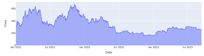

px.box(df, y='Close')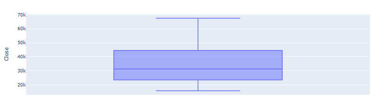

Box Cox Data Transformation

Applying the forward Box Cox transformation to the input data

bc= BoxCox()
df["Close"], lmbda =bc.transform_boxcox(df["Close"])

This is a statistical technique that transforms our target variable so that the transformed data closely resembles a normal distribution. In many statistical techniques, we assume that the errors are normally distributed. This assumption allows us to construct confidence intervals and conduct hypothesis tests implicit in Prophet.

Change of Variables

The input to Prophet is always a dataframe with two columns: ds and y. Therefore, we need to change the variables

data= df[["Date", "Close"]]
data.columns=["ds", "y"]

Here, the ds (date stamp) column should be of a format expected by Pandas, ideally YYYY-MM-DD for a date or YYYY-MM-DD HH:MM:SS for a timestamp. The y column must be numeric, and represents the measurement we wish to forecast (target).

Trend, Multi-Seasonal Decomposition & Forecast

Creating the Prophet model parameters

## Creating model parameters
model_param ={
    "daily_seasonality": False,
    "weekly_seasonality":False,
    "yearly_seasonality":True,
    "seasonality_mode": "multiplicative",
    "growth": "logistic"
}

Creating the model and setting a cap or upper limit for the forecast as we are using logistics growth

model = Prophet(**model_param)
data['cap']= data["y"].max() + data["y"].std() * 0.05 
# Setting a cap or upper limit for the forecast as we are using logistics growth
# The cap will be maximum value of target variable plus 5% of std.

Fitting the model and making the 1Y forecast in the (ds-y) domain

model.fit(data)
future= model.make_future_dataframe(periods=365)
future['cap'] = data['cap'].max()
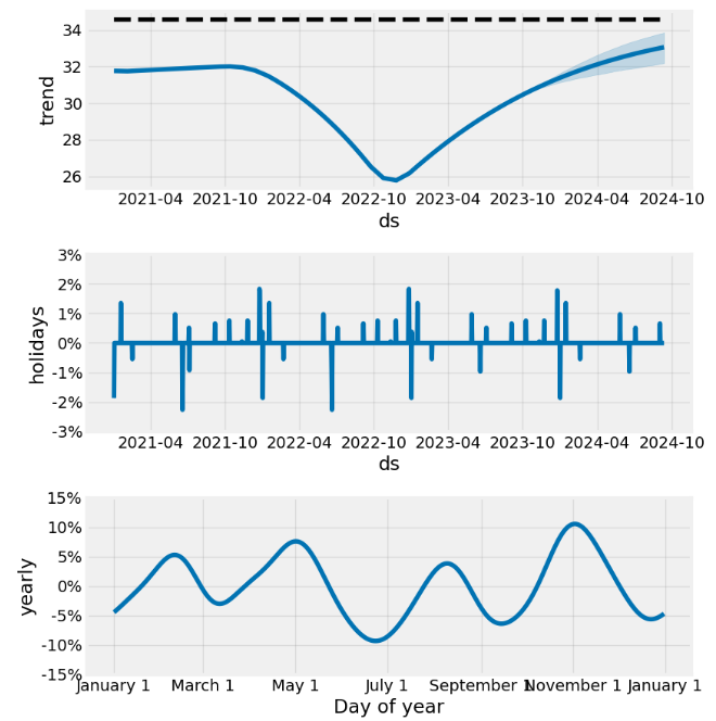
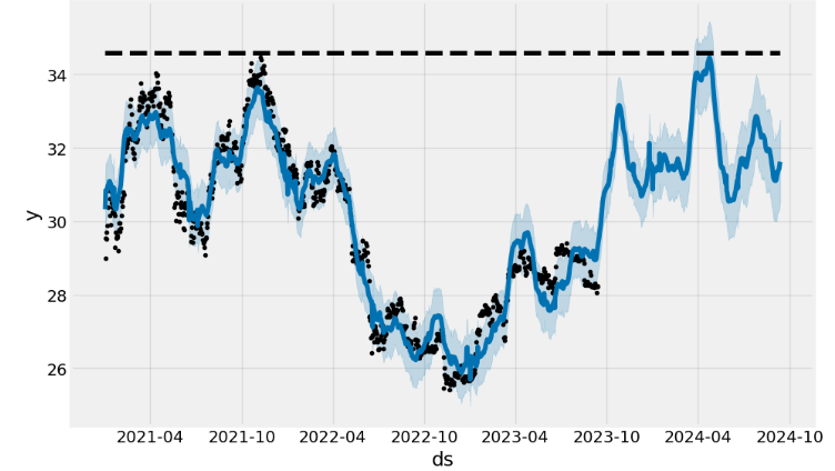
forecast= model.predict(future)

Plotting the trend, yearly seasonality, and forecast

model.plot_components(forecast);

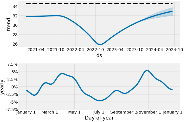
model.plot(forecast);# block dots are actual values and blue dots are forecast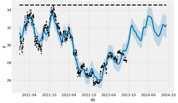

Adding monthly/quarterly seasonality and US events

model = Prophet(**model_param)

model= model.add_seasonality(name="monthly", period=30, fourier_order=10)
model= model.add_seasonality(name="quarterly", period=92.25, fourier_order=10)

model.add_country_holidays("US")

model.fit(data)

# Create future dataframe
future= model.make_future_dataframe(periods=365)
future['cap'] = data['cap'].max()

forecast= model.predict(future)

model.plot_components(forecast);
model.plot(forecast);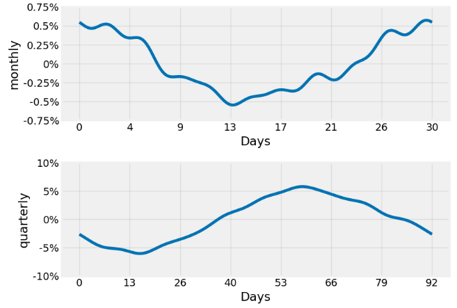

Trend, US holidays, and yearly seasonality

An interactive figure of the forecast and components can be created with plotly.
To get uncertainty in seasonality, we must do full Bayesian sampling.

Hyper-Parameter Tuning

Implementing the hyper-parameter model tuning

## Hyper parameter Tuning
import itertools
import numpy as np
from prophet.diagnostics import cross_validation, performance_metrics


param_grid={
    "daily_seasonality": [False],
    "weekly_seasonality":[False],
    "yearly_seasonality":[True],
    "growth": ["logistic"],
    'changepoint_prior_scale': [0.001, 0.01, 0.1, 0.5], # to give higher value to prior trend
    'seasonality_prior_scale': [0.01, 0.1, 1.0, 10.0] # to control the flexibility of seasonality components
}

# Generate all combination of parameters
all_params= [
            dict(zip(param_grid.keys(), v))
            for v in itertools.product(*param_grid.values())
]

print(all_params)

[{'daily_seasonality': False, 'weekly_seasonality': False, 'yearly_seasonality': True, 'growth': 'logistic', 'changepoint_prior_scale': 0.001, 'seasonality_prior_scale': 0.01}, {'daily_seasonality': False, 'weekly_seasonality': False, 'yearly_seasonality': True, 'growth': 'logistic', 'changepoint_prior_scale': 0.001, 'seasonality_prior_scale': 0.1}, {'daily_seasonality': False, 'weekly_seasonality': False, 'yearly_seasonality': True, 'growth': 'logistic', 'changepoint_prior_scale': 0.001, 'seasonality_prior_scale': 1.0}, {'daily_seasonality': False, 'weekly_seasonality': False, 'yearly_seasonality': True, 'growth': 'logistic', 'changepoint_prior_scale': 0.001, 'seasonality_prior_scale': 10.0}, {'daily_seasonality': False, 'weekly_seasonality': False, 'yearly_seasonality': True, 'growth': 'logistic', 'changepoint_prior_scale': 0.01, 'seasonality_prior_scale': 0.01}, {'daily_seasonality': False, 'weekly_seasonality': False, 'yearly_seasonality': True, 'growth': 'logistic', 'changepoint_prior_scale': 0.01, 'seasonality_prior_scale': 0.1}, {'daily_seasonality': False, 'weekly_seasonality': False, 'yearly_seasonality': True, 'growth': 'logistic', 'changepoint_prior_scale': 0.01, 'seasonality_prior_scale': 1.0}, {'daily_seasonality': False, 'weekly_seasonality': False, 'yearly_seasonality': True, 'growth': 'logistic', 'changepoint_prior_scale': 0.01, 'seasonality_prior_scale': 10.0}, {'daily_seasonality': False, 'weekly_seasonality': False, 'yearly_seasonality': True, 'growth': 'logistic', 'changepoint_prior_scale': 0.1, 'seasonality_prior_scale': 0.01}, {'daily_seasonality': False, 'weekly_seasonality': False, 'yearly_seasonality': True, 'growth': 'logistic', 'changepoint_prior_scale': 0.1, 'seasonality_prior_scale': 0.1}, {'daily_seasonality': False, 'weekly_seasonality': False, 'yearly_seasonality': True, 'growth': 'logistic', 'changepoint_prior_scale': 0.1, 'seasonality_prior_scale': 1.0}, {'daily_seasonality': False, 'weekly_seasonality': False, 'yearly_seasonality': True, 'growth': 'logistic', 'changepoint_prior_scale': 0.1, 'seasonality_prior_scale': 10.0}, {'daily_seasonality': False, 'weekly_seasonality': False, 'yearly_seasonality': True, 'growth': 'logistic', 'changepoint_prior_scale': 0.5, 'seasonality_prior_scale': 0.01}, {'daily_seasonality': False, 'weekly_seasonality': False, 'yearly_seasonality': True, 'growth': 'logistic', 'changepoint_prior_scale': 0.5, 'seasonality_prior_scale': 0.1}, {'daily_seasonality': False, 'weekly_seasonality': False, 'yearly_seasonality': True, 'growth': 'logistic', 'changepoint_prior_scale': 0.5, 'seasonality_prior_scale': 1.0}, {'daily_seasonality': False, 'weekly_seasonality': False, 'yearly_seasonality': True, 'growth': 'logistic', 'changepoint_prior_scale': 0.5, 'seasonality_prior_scale': 10.0}]

Adding seasonality, US events and finding the best hyper-parameters

rmses= list ()

# go through each combinations
for params in all_params:
    m= Prophet(**params)
    
    m= m.add_seasonality(name= 'monthly', period=15, fourier_order=5)
    m= m.add_seasonality(name= "quarterly", period= 30, fourier_order= 10)
    m.add_country_holidays(country_name="US")
    
    m.fit(data)
    

    df_cv= cross_validation(m, initial="365 days", period="30 days", horizon="365 days")
                            
    df_p= performance_metrics(df_cv, rolling_window=1)
                            
    rmses.append(df_p['rmse'].values[0])
                            
# find teh best parameters
best_params = all_params[np.argmin(rmses)]
                            
print("\n The best parameters are:", best_params) 

The best parameters are: {'daily_seasonality': False, 'weekly_seasonality': False, 'yearly_seasonality': True, 'growth': 'logistic', 'changepoint_prior_scale': 0.001, 'seasonality_prior_scale': 0.1} 

forecast.head()

 ds trend cap yhat_lower yhat_upper trend_lower trend_upper Christmas Day Christmas Day_lower Christmas Day_upper ... quarterly quarterly_lower quarterly_upper yearly yearly_lower yearly_upper additive_terms additive_terms_lower additive_terms_upper yhat
0 2021-02-04 27.956658 29.941582 27.135661 28.463372 27.956658 27.956658 0.0 0.0 0.0 ... -0.013422 -0.013422 -0.013422 0.008683 0.008683 0.008683 0.0 0.0 0.0 27.830485
1 2021-02-05 27.956395 29.941582 27.249080 28.605843 27.956395 27.956395 0.0 0.0 0.0 ... -0.012904 -0.012904 -0.012904 0.010045 0.010045 0.010045 0.0 0.0 0.0 27.921307
2 2021-02-06 27.956132 29.941582 27.357438 28.666751 27.956132 27.956132 0.0 0.0 0.0 ... -0.012104 -0.012104 -0.012104 0.011362 0.011362 0.011362 0.0 0.0 0.0 27.980221
3 2021-02-07 27.955869 29.941582 27.260377 28.679535 27.955869 27.955869 0.0 0.0 0.0 ... -0.011221 -0.011221 -0.011221 0.012609 0.012609 0.012609 0.0 0.0 0.0 28.036166
4 2021-02-08 27.955606 29.941582 27.461987 28.820484 27.955606 27.955606 0.0 0.0 0.0 ... -0.010445 -0.010445 -0.010445 0.013763 0.013763 0.013763 0.0 0.0 0.0 28.129553
5 rows × 74 columns

Inverse Box Cox Transformation

Applying the inverse Box Cox transformation to the forecast in the (ds-y) domain

forecast["yhat"]=bc.untransform_boxcox(x=forecast["yhat"], lmbda=lmbda)
forecast["yhat_lower"]=bc.untransform_boxcox(x=forecast["yhat_lower"], lmbda=lmbda)
forecast["yhat_upper"]=bc.untransform_boxcox(x=forecast["yhat_upper"], lmbda=lmbda)
forecast.plot(x="ds", y=["yhat_lower", "yhat", "yhat_upper"])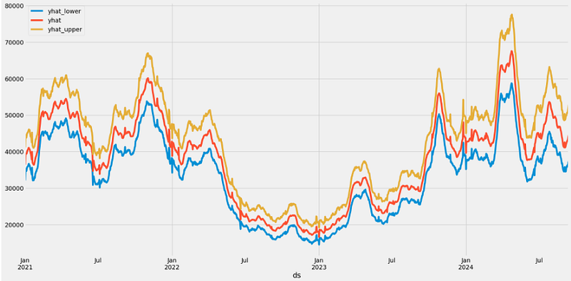

BTC-USD price forecast after the inverse Box Cox transformation

By default Prophet returns uncertainty intervals for the forecast yhat. The biggest source of uncertainty in the forecast is the potential for future trend changes. Here, we assume that the future will see similar trend changes as the history.

Conclusions

Recently, BTC has gained popularity among investors interested in the possibility of fast returns because it can be exchanged for and used in place of fiat currency.
In this post, we have addressed the very difficult task of predicting the highly volatile BTC price by invoking the state-of-the-art FB Prophet algorithm. The ultimate goal is to create algo-trading bots that learn to make money trading BTC.
One of the key advantages of Prophet over other models is its interpretability. Indeed, Prophet has been a key piece to improving Facebook’s ability to create a large number of trustworthy forecasts used for decision-making.
Generally, our results demonstrate the model’s effectiveness in capturing key trends and multi-seasonal fluctuations of BTC prices while accepting the uncertainties posed by the inherent volatility of the cryptocurrency market.
Note of caution: (1) if our dataset is noisy and does not follow business cycles, fine-tuning the model’s performance can be problematic; (2) Prophet provides an interpretable model with good performance in a short time; (3) although the model’s decisions are easy to interpret, it’s not precise enough to be used to measure the impact of an external event.
This Note does support the earlier QC studies.

BTC Price Prediction using FB Prophet

Basic Imports, Installations & Setups

Reading & Plotting Input Data

Box Cox Data Transformation

Change of Variables

Trend, Multi-Seasonal Decomposition & Forecast

Hyper-Parameter Tuning

Inverse Box Cox Transformation

Conclusions

Explore More

References

Contacts