for abuse survivors to internalize the lesson, “I’m bad” from their abuse, even when they are in no way at-fault.</p><p id="113b">In order to heal such unhealthy memories, we have to do two things. First, we need to learn to <i>desensitize</i> ourselves to the memories, so that they are no longer triggering. Second we need to <i>reprocess</i> them with a healthy belief about ourselves. By doing so, the sensory information from the memory can finally be paired with a healthy story of what happened. The memory, now whole, can finally be stored in long-term memory. The book can finally be closed and put away on the bookshelf where it belongs.</p><p id="c660" type="7">This is why traumatic memories can still feel so vivid even when they happened a long time ago.</p><figure id="8c71"><img src="https://cdn-images-1.readmedium.com/v2/resize:fit:800/1*vGddg7i-Npz35GlTuEJhNA.png"><figcaption>The left image shows over-active brain activity of a client with Post-Traumatic Stress. The right scan shows brain activity after EMDR treatment. Credit: Dr. Daniel Amen.</figcaption></figure><p id="cec8">Research has shown that one way to help desensitize and reprocess memories is by alternately stimulating the left and right-hand sides of the brain. One way to do this is by moving the eyes to the left and right, something that, remarkably, happens naturally as we sleep. Another way is to alternately tap on the left and right hand sides of the body, for example on the hands or knees. Treatment that utilizes these techniques is known as Eye-Movement Desensitization and Reprocessing, or EMDR. While originally developed for the treatment of trauma, EMDR can also be effective <a href="https://www.emdr.com/research-overview/#adaptive">for many other chronic, “stuck” issues such as anxiety, depression, phobias, or body image</a>.</p><figure id="d73c"><img src="https://cdn-images-1.readmedium.com/v2/resize:fit:800/1*hkBFbyd8f229q6w97-jAaA.jpeg"><figcaption>Photo: JuergenPM / pixabay.com</figcaption></figure><p id="2924">A first step of EMDR treatment is to equip you with tools and techniques that empower you to manage your arousal. Only when you feel proficient with these tools do you move on to processing past memories at a pace that feels safe to you.</p><p id="04f2">At the conclusion of EMDR treatment, the goal is being able to merely <i>recall</i> these memories rather than being forced to <i>re-live</i> them, to merely <i>have</i> memories rather than feeling like the memories
Options
<i>have you</i>.</p><p id="6a0a"><b><i>Peter W. Pruyn</i></b><i> (“prine”) is a psychotherapist in Northampton, Massachusetts, a member of the New England Society for the Treatment of Trauma and Dissociation (<a href="https://www.nesttd-online.org/">NESTTD</a>), and author of <a href="https://www.etsy.com/listing/993937295/peters-psycho-ed-handouts-client"></a></i><a href="https://www.etsy.com/listing/993937295/peters-psycho-ed-handouts-client">Peter’s Psycho-Ed Handouts: Client Handouts and Therapist Resources for Trauma, EMDR, and General Psychotherapy</a>.</p><p id="ec8f"><i>For more by this author, try:</i></p><div id="b546" class="link-block">
<a href="https://readmedium.com/how-to-find-a-good-emdr-therapist-8164e38fc79f">
<div>
<div>
<h2>How to Find a Good EMDR Therapist</h2>
<div><h3>Ten tips to help you decided whether a trauma therapist is right for you</h3></div>
<div><p>medium.com</p></div>
</div>
<div>
<div style="background-image: url(https://miro.readmedium.com/v2/resize:fit:320/1*G81sywTnCEHzho-kZFMuJg.jpeg)"></div>
</div>
</div>
</a>
</div><div id="0a0d" class="link-block">
<a href="https://readmedium.com/treating-endometriosis-with-emdr-5d3898240e0">
<div>
<div>
<h2>Treating Endometriosis Pain with EMDR</h2>
<div><h3>Healing our stories can lessen our pain</h3></div>
<div><p>medium.com</p></div>
</div>
<div>
<div style="background-image: url(https://miro.readmedium.com/v2/resize:fit:320/1*jdQmiOk7bWGTr9BHUxzskA.png)"></div>
</div>
</div>
</a>
</div><div id="408c" class="link-block">
<a href="https://readmedium.com/why-a-trauma-therapist-recommends-chessy-prouts-story-e087ba4d8106">
<div>
<div>
<h2>Why a Trauma Therapist Recommends Chessy Prout’s Story</h2>
<div><h3>Empowerment + Connection → Recovery from Sexual Assault</h3></div>
<div><p>medium.com</p></div>
</div>
<div>
<div style="background-image: url(https://miro.readmedium.com/v2/resize:fit:320/1*85urCfNAUhdLFNrWJX3pAw.jpeg)"></div>
</div>
</div>
</a>
</div></article></body>
Backtesting the NVIDIA Scalping Strategy with SPY Benchmark & VaR Simulations
In this post, the focus is on 1Y backtesting the NVIDIA (NASDAQ: NVDA) scalping algo-trading strategy as compared to the buy-hold strategy and the SPY ETF benchmark. In addition, we’ll quantify the potential risk of loss by running stochastic simulations for computing the Value-at-Risk (VaR).
Challenge 2: NVDA, the tech behemoth, definitely tempts as a day trading option, but let’s be real — you’ll want to find stocks that are easy to buy and sell (that’s called liquidity), don’t burn you with high transaction fees, swing enough in price to make things interesting (hello, volatility), and have enough people trading them to ensure there’s always a buyer or seller when you need one.
Solution Part 1: Scalping is a day trading technique where an investor buys and sells an individual stock multiple times throughout the same day. Scalpers seek to profit from small market movements, taking advantage of a ticker tape that never stands still.
Solution Part 2: VaR serves as a tool to quantify investment risks by providing estimates of maximum potential losses given a certain level of confidence in making predictions about stock returns within a specific timeframe.
Let’s begin with basic settings and imports:
import os
os.chdir('YOURPATH') # Set working directory
os. getcwd()
# IMPORTING PACKAGESimport requests
import pandas as pd
import matplotlib.pyplot as plt
from termcolor import colored as cl
import numpy as np
import math
Calculating the intraday open-close % price change
# CALCULATING % CHANGE
nvd['pclose_open_pc'] = np.nan
for i inrange(1, len(nvd)):
diff, avg = (nvd.close[i-1] - nvd.open[i]) , (nvd.close[i-1] + nvd.open[i])/2
pct_change = (diff / avg)*100
nvd['pclose_open_pc'][i] = pct_change
nvd = nvd[nvd.pclose_open_pc > 1]
nvd.tail()
open high low close volume pclose_open_pc
datetime
2024-03-19867.00000905.44000850.09998893.9799867217100.02.0039382024-04-02 884.47998900.94000876.20001894.5200243306400.02.1419292024-04-03 884.84003903.73999884.00000889.6400137006700.01.0880302024-04-10839.26001874.00000837.09003870.3900143192900.01.6871422024-04-12896.98999901.75000875.29999881.8599942488900.01.017107
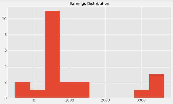
Extracting the intraday stock data, defining the entering/exiting position, and calculating the day trade earnings by investing $10k
investment = 10000
equity = investment
earning = 0
earnings_record = []
for i inrange(len(nvd)):
# EXTRACTING INTRADAY DATA
date = str(nvd.index[i])[:10]
# ENTERING POSITION
open_p = nvd.iloc[i].open
no_of_shares = math.floor(equity/open_p)
equity -= (no_of_shares * open_p)
# EXITING POSITION
nvd['p_change'] = np.nan
for i inrange(len(nvd)):
diff, avg = (nvd.close[i] - open_p), (nvd.close[i] + open_p)/2
pct_change = (diff / avg)*100
nvd['p_change'][i] = pct_change
nvd = nvd.dropna()
greater_1 = nvd[nvd.p_change > 1]
iflen(greater_1) > 0:
sell_price = greater_1.iloc[0].close
equity += (no_of_shares * sell_price)
else:
sell_price = nvd.iloc[-1].close
equity += (no_of_shares * sell_price)
# CALCULATING TRADE EARNINGS
investment += earning
earning = round(equity-investment, 2)
earnings_record.append(earning)
if earning > 0:
print(cl('PROFIT:', color = 'green', attrs = ['bold']), f'Earning on {date}: ${earning}; Bought ', cl(f'{no_of_shares}', attrs = ['bold']), 'stocks at ', cl(f'${open_p}', attrs = ['bold']), 'and Sold at ', cl(f'${sell_price}', attrs = ['bold']))
else:
print(cl('LOSS:', color = 'red', attrs = ['bold']), f'Loss on {date}: ${earning}; Bought ', cl(f'{no_of_shares}', attrs = ['bold']), 'stocks at ', cl(f'${open_p}', attrs = ['bold']), 'and Sold at ', cl(f'${sell_price}', attrs = ['bold']))
PROFIT: Earning on 2023-10-06: $345.18; Bought 22 stocks at $441.92999and Sold at $457.62
PROFIT: Earning on 2023-10-09: $211.6; Bought 23 stocks at $448.42001and Sold at $457.62
PROFIT: Earning on 2023-10-17: $405.26; Bought 23 stocks at $440.0and Sold at $457.62
PROFIT: Earning on 2023-10-18: $792.75; Bought 25 stocks at $425.91and Sold at $457.62
PROFIT: Earning on 2023-10-31: $1540.48; Bought 29 stocks at $404.5and Sold at $457.62
PROFIT: Earning on 2023-12-04: $442.4; Bought 28 stocks at $460.76999and Sold at $476.57001
PROFIT: Earning on 2023-12-12: $467.19; Bought 29 stocks at $460.45999and Sold at $476.57001
PROFIT: Earning on 2023-12-19: $3249.96; Bought 28 stocks at $494.23999and Sold at $610.31
PROFIT: Earning on 2024-01-03: $762.84; Bought 36 stocks at $474.85001and Sold at $496.04001
PROFIT: Earning on 2024-01-26: $3238.72; Bought 29 stocks at $609.59998and Sold at $721.28003
PROFIT: Earning on 2024-01-31: $3633.92; Bought 34 stocks at $614.40002and Sold at $721.28003
PROFIT: Earning on 2024-02-13: $604.8; Bought 35 stocks at $704.0and Sold at $721.28003
PROFIT: Earning on 2024-02-21: $1525.15; Bought 37 stocks at $680.06and Sold at $721.28003
PROFIT: Earning on 2024-02-28: $2853.89; Bought 35 stocks at $776.20001and Sold at $857.73999
PROFIT: Earning on 2024-03-11: $515.11; Bought 34 stocks at $864.28998and Sold at $879.44
LOSS: Loss on 2024-03-14: $-472.95; Bought 34 stocks at $895.77002and Sold at $881.85999
PROFIT: Earning on 2024-03-15: $344.76; Bought 34 stocks at $869.29999and Sold at $879.44
PROFIT: Earning on 2024-03-19: $435.4; Bought 35 stocks at $867.0and Sold at $879.44
PROFIT: Earning on 2024-04-02: $323.0; Bought 34 stocks at $884.47998and Sold at $893.97998
PROFIT: Earning on 2024-04-03: $319.9; Bought 35 stocks at $884.84003and Sold at $893.97998
PROFIT: Earning on 2024-04-10: $683.76; Bought 37 stocks at $839.26001and Sold at $857.73999
LOSS: Loss on 2024-04-12: $-529.55; Bought 35 stocks at $896.98999and Sold at $881.85999
initial_price =prices.iloc[-1] # Use the last price as the initial price
num_simulations = 400# Number of simulations
confidence_level = 0.95# Confidence level for VaR estimation
duration = 260
Running the random simulations and calculating VaR
price_paths = np.zeros((num_simulations,duration))
for i inrange(num_simulations):
price_paths[i, 0] = initial_price
for day inrange(1, duration):
drift = mean_return * (1 / duration)
shock = volatility * np.random.randn() * np.sqrt(1 / duration)
price_paths[i, day] = price_paths[i, day - 1] * (1 + drift + shock)
# Calculate daily returns for each simulation
returns = (price_paths[:, 1:] - price_paths[:, :-1]) / price_paths[:, :-1]
# Calculate the portfolio value at the end of 2023
portfolio_value = 10000# Example portfolio value
portfolio_returns = portfolio_value * returns
# Calculate the VaR
sorted_portfolio_returns = np.sort(portfolio_returns)
var_index = int(num_simulations * (1 - confidence_level))
var = -sorted_portfolio_returns[var_index]
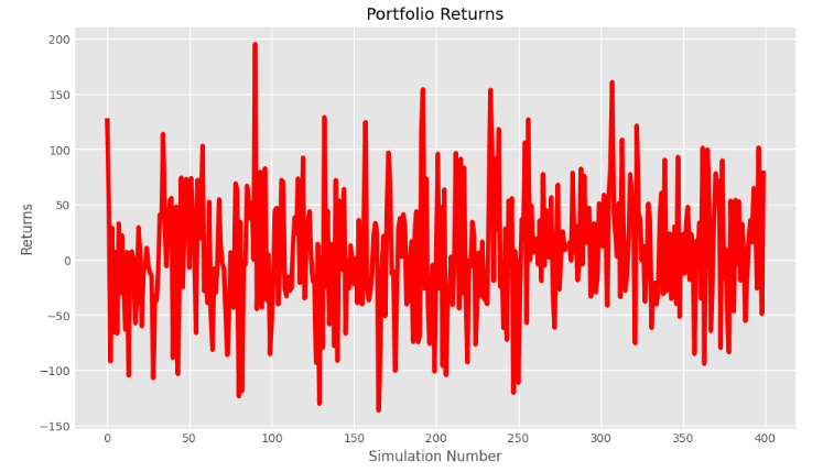
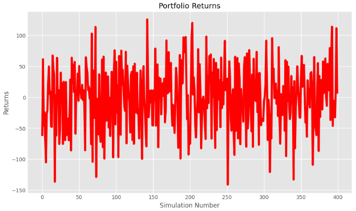
Plotting slices of the portfolio returns 2D array
print(portfolio_returns.shape)
(400, 259)

port1=portfolio_returns[:,0]
x = np.arange(0, 400)
y=port1
# plotting
plt.figure(figsize=(10,6))
plt.title("Portfolio Returns")
plt.xlabel("Simulation Number")
plt.ylabel("Returns")
plt.plot(x, y, color ="red")
plt.show()
Portfolio Returns vs Simulation Number: Time Slot 1
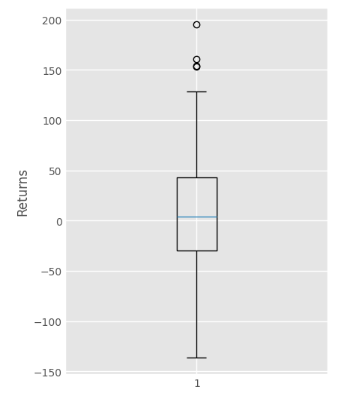
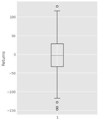
# Creating plot
plt.figure(figsize=(4,6))
plt.boxplot(port1)
plt.ylabel("Returns")
# show plot
plt.show()
Portfolio Returns Box Plot: Time Slot 1
port1=portfolio_returns[:,250]
x = np.arange(0, 400)
y=port1
# plotting
plt.figure(figsize=(10,6))
plt.title("Portfolio Returns")
plt.xlabel("Simulation Number")
plt.ylabel("Returns")
plt.plot(x, y, color ="red")
plt.show()
Portfolio Returns vs Simulation Number: Time Slot 249
# Creating plot
plt.figure(figsize=(4,6))
plt.boxplot(port1)
plt.ylabel("Returns")
# show plot
plt.show()
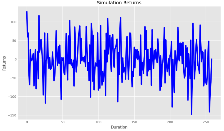
port11=portfolio_returns[0,:]
x = np.arange(0, 259)
y=port11
# plotting
plt.figure(figsize=(10,6))
plt.title("Simulation Returns")
plt.xlabel("Duration")
plt.ylabel("Returns")
plt.plot(x, y, color ="blue")
plt.show()
Returns vs Duration: Simulation 1
# Creating plot
plt.figure(figsize=(4,6))
plt.boxplot(port11)
plt.ylabel("Returns")
# show plot
plt.show()
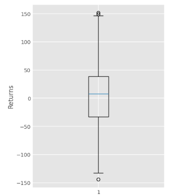
Returns Box Plot: Simulation 1
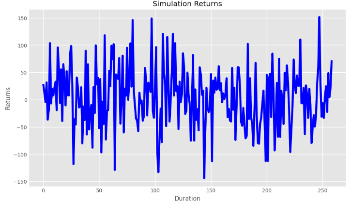
port11=portfolio_returns[300,:]
x = np.arange(0, 259)
y=port11
# plotting
plt.figure(figsize=(10,6))
plt.title("Simulation Returns")
plt.xlabel("Duration")
plt.ylabel("Returns")
plt.plot(x, y, color ="blue")
plt.show()
Returns vs Duration: Simulation 299
# Creating plot
plt.figure(figsize=(4,6))
plt.boxplot(port11)
plt.ylabel("Returns")
# show plot
plt.show()
Returns Box Plot: Simulation 299
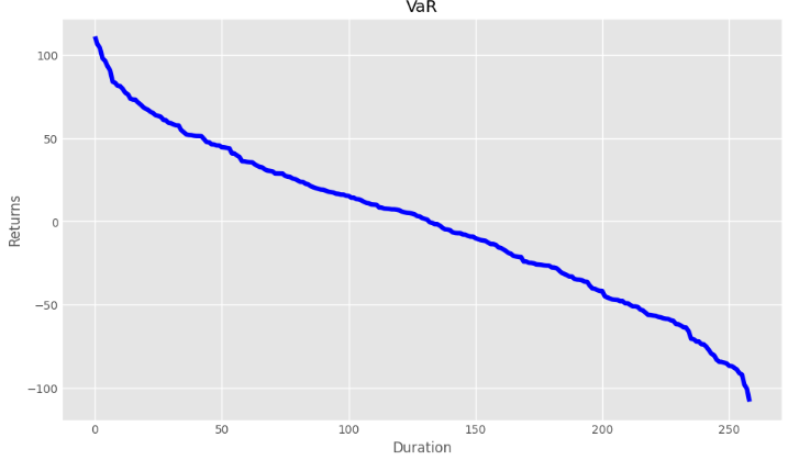
Plotting VaR: Returns vs Duration
x = np.arange(0, 259)
y=var
# plotting
plt.figure(figsize=(10,6))
plt.title("VaR")
plt.xlabel("Duration")
plt.ylabel("Returns")
plt.plot(x, y, color ="blue")
plt.show()
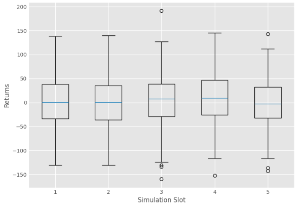
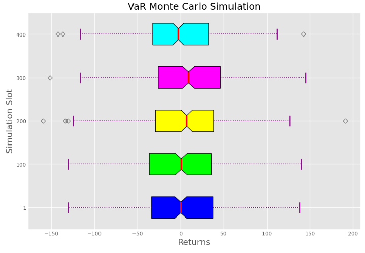
Customized box plots Returns vs Simulation Slots 1–5
data = [data_1, data_2, data_3, data_4, data_5]
fig = plt.figure(figsize =(10, 7))
ax = fig.add_subplot(111)
# Creating axes instance
bp = ax.boxplot(data, patch_artist = True,
notch ='True', vert = 0)
colors = ['#0000FF', '#00FF00',
'#FFFF00', '#FF00FF','#00FFFF']
for patch, color inzip(bp['boxes'], colors):
patch.set_facecolor(color)
# changing color and linewidth of# whiskersfor whisker in bp['whiskers']:
whisker.set(color ='#8B008B',
linewidth = 1.5,
linestyle =":")
# changing color and linewidth of# capsfor cap in bp['caps']:
cap.set(color ='#8B008B',
linewidth = 2)
# changing color and linewidth of# mediansfor median in bp['medians']:
median.set(color ='red',
linewidth = 3)
# changing style of fliersfor flier in bp['fliers']:
flier.set(marker ='D',
color ='#e7298a',
alpha = 0.5)
# x-axis labels
ax.set_yticklabels(['1', '100',
'200', '300','400'])
# Adding title
plt.title("VaR Monte Carlo Simulation",fontsize=18)
plt.xlabel("Returns",fontsize=16)
plt.ylabel("Simulation Slot",fontsize=16)
# Removing top axes and right axes# ticks
ax.get_xaxis().tick_bottom()
ax.get_yaxis().tick_left()
# show plot
plt.show()
Customized box plots Returns vs Simulation Slots 1–5
Conclusions
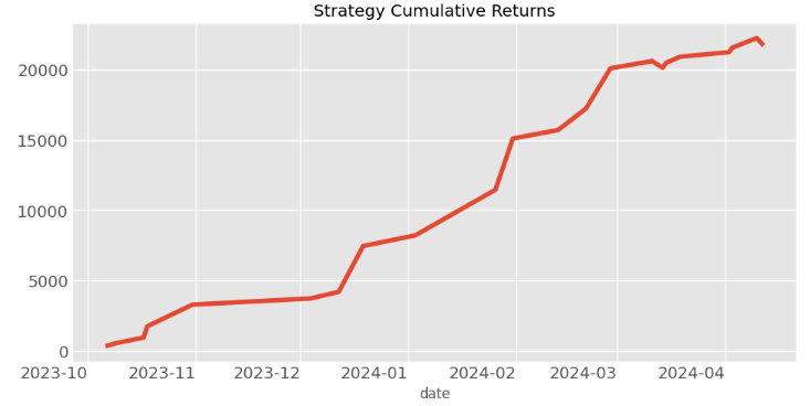
The NVDA 2023–24 backtesting results by investing $10k are as follows: EARNING: $21693.57 ; ROI: 216.94%
MAX LOSS: $-529.55; MAX PROFIT: 3633.92; TOTAL TRADES: 22; WIN RATE: 91%; AVG. TRADES/MONTH: 0; AVG. EARNING/MONTH: $181
BUY/HOLD STRATEGY ROI: 73.25%
Benchmark profit by investing $10k : 1587.26
Benchmark Profit percentage : 15%
Scalping Strategy profit is201.94% higher than the Benchmark Profit
The estimated volatility is 0.085 and mean return is 0.035.
We have shown that NVDA scalping can be a profitable trading approach with a 91% win rate but requires careful risk management, algo-trading backtesting and benchmarking.