
BTC-USD Price Prediction using FB Prophet with Hyperparameter Optimization, Cross-Validation QC & Modified Algo-Trading Strategies

- This post is a continuation of our previous study aimed at developing a detailed framework for BTC-USD price prediction using Facebook’s Prophet implemented in Python [1–5] (v.i. Resources).
- The present comparative analysis provides a more detailed look at option testing and model tuning or Hyperparameter Optimization (HPO) based on functionality for time series cross validation QC to measure forecast error using historical data.
- In addition to simulated BTC forecasts, we’ll explain in detail how we can use FB Prophet to optimize crypto algo-trading strategies as compared to Buy & Hold benchmark. Read more details here.
Business Case
- Proper cryptocurrency forecasting can lead to great profits combined with effective risk management for crypto traders.
- Recently, BTC has been the subject of many price predictions.
- CoinCodex: Based on the historical price movements of BTC and the BTC halving cycles, BTC could gain 201.59% by 2025 if BTC reaches the upper price target. Meanwhile, the price of BTC is predicted to reach as high as $ 173,833 next year.
- But will the price of Bitcoin hit $1 million by 2030?
About FB Prophet
- FB Prophet is a procedure for forecasting time series data based on trend/seasonality modelling and Bayesian inference.
- It works best with time series that have strong seasonal effects and is robust to missing data, outliers and shifts in the trend.
- The forecast model consists of the following 4 components: trends (changes over a long period of time), seasonality (periodic or short-term changes), holidays, and unconditional changes that is specific to a business.
- It is specially interesting for new users because of its easy use and capacity of find automatically a good set of hyperparameters for the model.
- Examples include additional regressors, multiplicative seasonality, non-daily data, measuring uncertainty and diagnostics.
Let’s delve into the specifics of BTC-USD price prediction using this library.
Key Installations
pip is our preferred installer program. Starting with Python 3.4, it is included by default with the Python binary installers.- Launching Jupyter Notebook and installing the essential Python libraries
!pip install statsmodels, math, yfinance, prophet, plotly,matplotlib, itertools
Imports & Settings
- Make sure that we have necessary libraries & dependencies available to run the code successfully
import pandas as pd
import plotly.express as px
import requests
import numpy as np
import matplotlib.pyplot as plt
from math import floor
from termcolor import colored as cl
import yfinance as yf
import datetime
from datetime import date, timedelta

# Import Prophet
from prophet import Prophet

plt.rcParams['figure.figsize'] = (12, 6)
plt.style.use('fivethirtyeight')

import os
os.chdir('YOURPATH')    # Set working directory
os. getcwd()
Input Stock Data
- Reading the input BTC-USD historical data with days=730
today = date.today()

d1 = today.strftime("%Y-%m-%d")
end_date = d1
d2 = date.today() - timedelta(days=730)
d2 = d2.strftime("%Y-%m-%d")
start_date = d2

data = yf.download('BTC-USD',
                      start=start_date,
                      end=end_date,
                      progress=False)
data["Date"] = data.index
data = data[["Date", "Open", "High", "Low", "Close", "Adj Close", "Volume"]]
data.reset_index(drop=True, inplace=True)
data.tail()

Date           Open      High      Low       Close     Adj Close  Volume
725 2024-07-02 62,844.41 63,203.36 61,752.75 62,029.02 62,029.02 20151616992
726 2024-07-03 62,034.33 62,187.70 59,419.39 60,173.92 60,173.92 29756701685
727 2024-07-04 60,147.14 60,399.68 56,777.80 56,977.70 56,977.70 41149609230
728 2024-07-05 57,022.81 57,497.15 53,717.38 56,662.38 56,662.38 55417544033
729 2024-07-06 56,659.07 58,472.55 56,038.96 58,303.54 58,303.54 20610320577- Plotting the Close price
plt.plot(data['Date'],data['Close'])
plt.xlabel('Date')
plt.ylabel('Close Price USD')
plt.title('BTC-USD Close Price')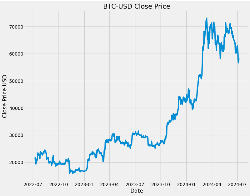
Data Preparation
- Applying the Box Cox transformation to transform the non-normal dependent Close price into a normal shape
### Box Cox transformation
from statsmodels.base.transform import BoxCox

bc= BoxCox()
data["Close"], lmbda =bc.transform_boxcox(data["Close"])- Creating the input to Prophet
data1=data[["Date", "Close"]]
data1.columns=["ds", "y"]

data1.tail()

    ds          y
725 2024-07-02 42.381398
726 2024-07-03 42.086488
727 2024-07-04 41.560999
728 2024-07-05 41.507898
729 2024-07-06 41.781750- The input to Prophet is always a dataframe with two columns: ds and y . The ds (datestamp) column should be of a format expected by Pandas, ideally YYYY-MM-DD for a date or YYYY-MM-DD HH:MM:SS for a timestamp. The y column must be numeric, and represents the measurement we wish to forecast.
Prophet with Max Cap & 5% STD
- Creating the list of model parameters with yearly multiplicative seasonality and logistic growth
model_param ={
    "daily_seasonality": False,
    "weekly_seasonality":False,
    "yearly_seasonality":True,
    "seasonality_mode": "multiplicative",
    "growth": "logistic"
}- By default, Prophet fits additive seasonality, meaning the effect of the seasonality is added to the trend to get the forecast. In the above model, the seasonality is not a constant additive factor as assumed by Prophet, rather it grows with the trend. This is multiplicative seasonality.
- By default, Prophet uses a linear model for its forecast. When forecasting growth, there is usually some maximum achievable point: total market size, etc. This is called the carrying capacity, and the forecast should saturate at this point. Prophet allows us to make forecasts using a logistic growth trend model, with a specified carrying capacity.
- Running the model
model = Prophet(**model_param)
- Setting a cap or upper limit for the forecast as we are using logistics growth. The cap will be maximum value of price plus 5% of STD
data1['cap']= data1["y"].max() + data1["y"].std() * 0.05 - Fitting the model
model.fit(data1)
- Creating the in-sample & 1Y out-of-sample forecast with the above cap
future= model.make_future_dataframe(periods=365)

future['cap'] = data1['cap'].max()

forecast= model.predict(future)- Plotting the (ds-y) domain prediction with key components
model.plot(forecast,figsize=(14, 8))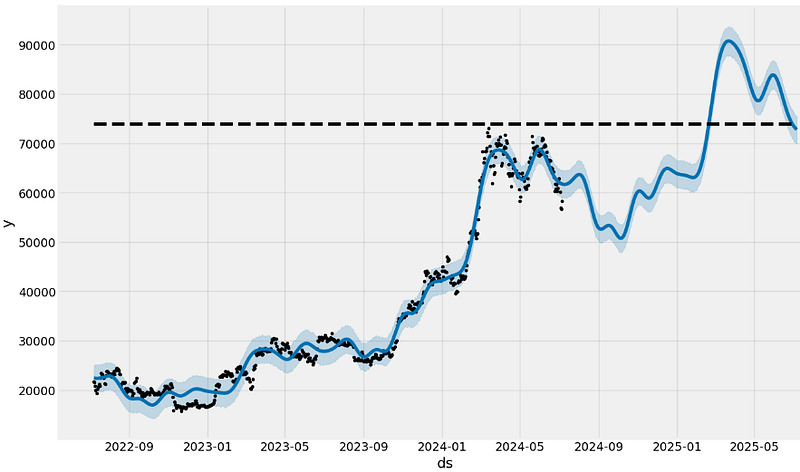
model.plot_components(forecast,figsize=(16, 10));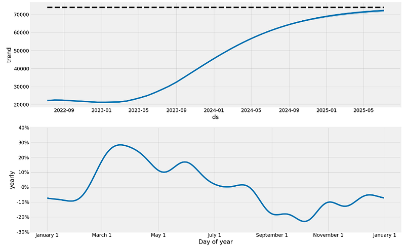
Prophet with Monthly/Quarterly Seasonality & US Holidays
- Running Prophet with monthly/quarterly seasonality and US holidays
model = Prophet(**model_param)
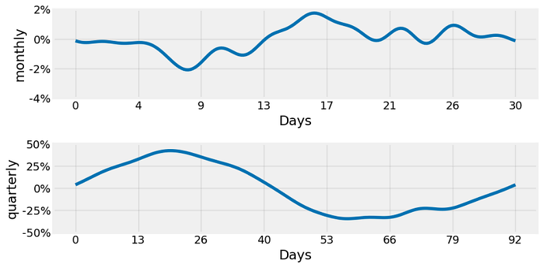
model= model.add_seasonality(name="monthly", period=30, fourier_order=10)
model= model.add_seasonality(name="quarterly", period=92.25, fourier_order=10)
model.add_country_holidays("US")
model.fit(data1)
# Create future dataframe
future= model.make_future_dataframe(periods=365)
future['cap'] = data1['cap'].max()
forecast= model.predict(future)
from prophet.plot import plot
plot(model, forecast, figsize=(14, 8))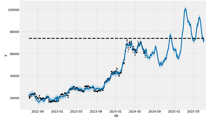
from prophet.plot import plot_components

plot_components(model, forecast, figsize=(10, 12))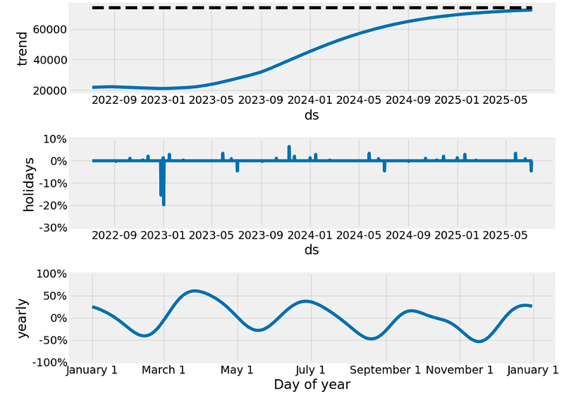
- Performing the inverse Box-Cox transformation to get the original price
forecast["yhat"]=bc.untransform_boxcox(x=forecast["yhat"], lmbda=lmbda)
forecast["yhat_lower"]=bc.untransform_boxcox(x=forecast["yhat_lower"], lmbda=lmbda)
forecast["yhat_upper"]=bc.untransform_boxcox(x=forecast["yhat_upper"], lmbda=lmbda)
forecast.plot(x="ds", y=["yhat_lower", "yhat", "yhat_upper"])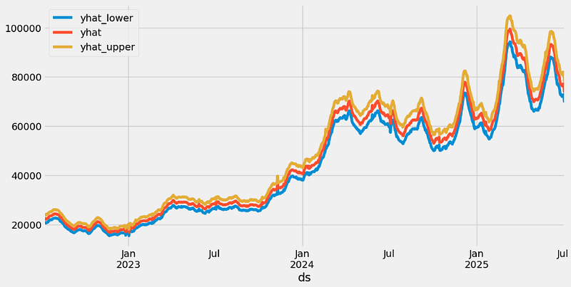
- Computing some useful statistics of the prediction performance with manually selected cutoffs
from prophet.diagnostics import cross_validation, performance_metrics
from prophet.plot import plot_cross_validation_metric
df_cv = cross_validation(model, initial="600 days", period="30 days", horizon="90 days")
cutoffs = pd.to_datetime(['2022-09-01', '2023-05-01', '2024-03-01'])
df_cv2 = cross_validation(model, cutoffs=cutoffs, horizon='90 days')
fig = plot_cross_validation_metric(df_cv2, metric='rmse')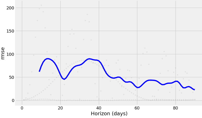
- Printing the summary of performance metrics
df_p = performance_metrics(df_cv2)
df_p.head()

    horizon mse      rmse       mae       mape     mdape   smape coverage
0 9 days 3805.462369 61.688430 29.520999 0.893692 0.118312 0.355870 0.0
1 10 days 5382.793620 73.367524 37.768231 1.140719 0.168333 0.425770 0.0
2 11 days 6754.735216 82.187196 45.409934 1.368028 0.286148 0.491224 0.0
3 12 days 7678.053041 87.624500 51.465541 1.551664 0.352840 0.546114 0.0
4 13 days 8071.329465 89.840578 55.027843 1.658574 0.426625 0.584601 0.0
- Plotting MAPE
fig = plot_cross_validation_metric(df_cv2, metric='mape')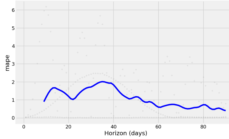
- Plotting MAE
fig = plot_cross_validation_metric(df_cv2, metric='mae')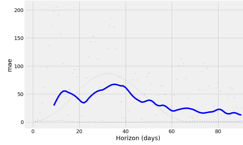
Hyperparameter Optimization (HPO)
- Running HPO by adding monthly/quarterly seasonality and US holidays
rmses= list ()

# go through each combinations
for params in all_params:
    m= Prophet(**params)

    m= m.add_seasonality(name= 'monthly', period=30, fourier_order=5)
    m= m.add_seasonality(name= "quarterly", period= 92.25, fourier_order= 10)


    m.add_country_holidays(country_name="US")

    m.fit(data1)

    df_cv= cross_validation(m, initial="500 days", period="180 days", horizon="90 days")

    df_p= performance_metrics(df_cv, rolling_window=1)

    rmses.append(df_p['rmse'].values[0])

# find teh best parameters
best_params = all_params[np.argmin(rmses)]

print("\n The best parameters are:", best_params)

The best parameters are: {'daily_seasonality': False, 'weekly_seasonality': False, 'yearly_seasonality': True, 'growth': 'logistic', 'changepoint_prior_scale': 0.01, 'seasonality_prior_scale': 0.01} - Fitting the optimized model and creating the corresponding forecast
model_param1 ={
    "daily_seasonality": False,
    "weekly_seasonality":False,
    "yearly_seasonality":True,
    "seasonality_mode": "multiplicative",
    "growth": "logistic",
    'seasonality_prior_scale': 0.1,
    'changepoint_prior_scale': 0.01
}

model1 = Prophet(**model_param1)


model1.add_country_holidays("US")

model1.fit(data1)

# Create future dataframe
future= model1.make_future_dataframe(periods=365)
future['cap'] = data1['cap'].max()

forecast= model1.predict(future)- Applying the inverse Box-Cox transform to get original prices
forecast["yhat"]=bc.untransform_boxcox(x=forecast["yhat"], lmbda=lmbda)
forecast["yhat_lower"]=bc.untransform_boxcox(x=forecast["yhat_lower"], lmbda=lmbda)
forecast["yhat_upper"]=bc.untransform_boxcox(x=forecast["yhat_upper"], lmbda=lmbda)
forecast.plot(x="ds", y=["yhat_lower", "yhat", "yhat_upper"])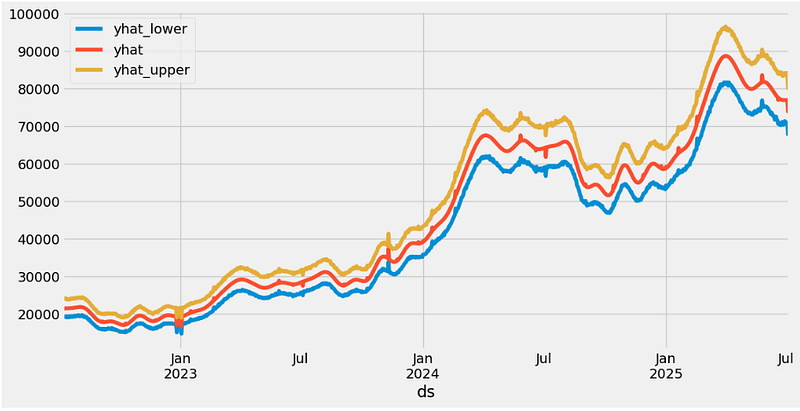
- Running cross-validation QC with manual cutoffs
cutoffs = pd.to_datetime(['2022-09-01', '2023-05-01', '2024-03-01'])
df_cv2 = cross_validation(model1, cutoffs=cutoffs, horizon='90 days')
fig = plot_cross_validation_metric(df_cv2, metric='rmse')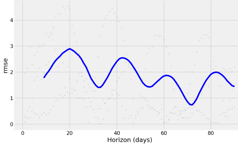
fig = plot_cross_validation_metric(df_cv2, metric='mape')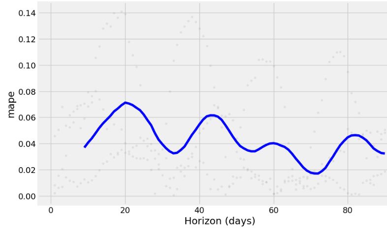
fig = plot_cross_validation_metric(df_cv2, metric='mae')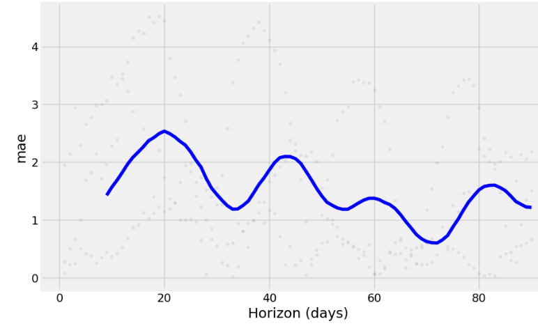
Preparing BTC-USD Historical Data 2020–2024
- Preparing the BTC-USD historical data from 2020–01–01 to 2024–07–07 without the Box-Cox transformation
import pandas as pd
import numpy as np
from prophet import Prophet
import matplotlib.pyplot as plt
from functools import reduce

%matplotlib inline
import warnings
warnings.filterwarnings('ignore')

pd.options.display.float_format = "{:,.2f}".format

import yfinance as yf

ticker = 'BTC-USD'
start_date = '2020-01-01'


stock_price = yf.download(ticker, start=start_date)
stock_price["Date"] = stock_price.index
stock_price.tail()

           Open      High      Low       Close    Adj Close   Volume      Date
Date
2024-07-03 62,034.33 62,187.70 59,419.39 60,173.92 60,173.92 29756701685 2024-07-03
2024-07-04 60,147.14 60,399.68 56,777.80 56,977.70 56,977.70 41149609230 2024-07-04
2024-07-05 57,022.81 57,497.15 53,717.38 56,662.38 56,662.38 55417544033 2024-07-05
2024-07-06 56,659.07 58,472.55 56,038.96 58,303.54 58,303.54 20610320577 2024-07-06
2024-07-07 58,239.43 58,367.18 56,644.89 57,198.04 57,198.04 19585976320 2024-07-07

stock_price = stock_price[['Date','Adj Close']]

stock_price.columns = ['ds', 'y']
stock_price.tail()

           ds          y
Date
2024-07-03 2024-07-03 60,173.92
2024-07-04 2024-07-04 56,977.70
2024-07-05 2024-07-05 56,662.38
2024-07-06 2024-07-06 58,303.54
2024-07-07 2024-07-07 57,198.04- Fitting the default Prophet model and creating the forecast until 2027–07–07
model = Prophet()
model.fit(stock_price)
future = model.make_future_dataframe(1095, freq='d')

future_boolean = future['ds'].map(lambda x : True if x.weekday() in range(0, 5) else False)
future = future[future_boolean]

future.tail()
ds
2738 2027-07-01
2739 2027-07-02
2742 2027-07-05
2743 2027-07-06
2744 2027-07-07

forecast = model.predict(future)
#forecast.tail()

model.plot(forecast);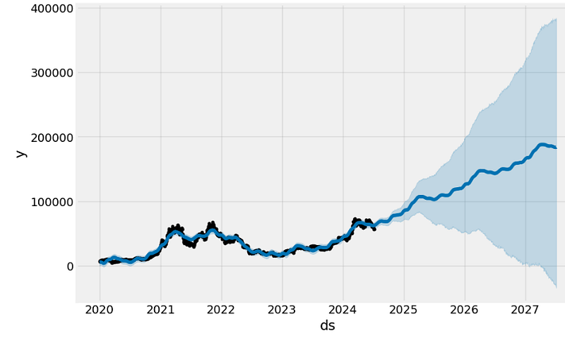
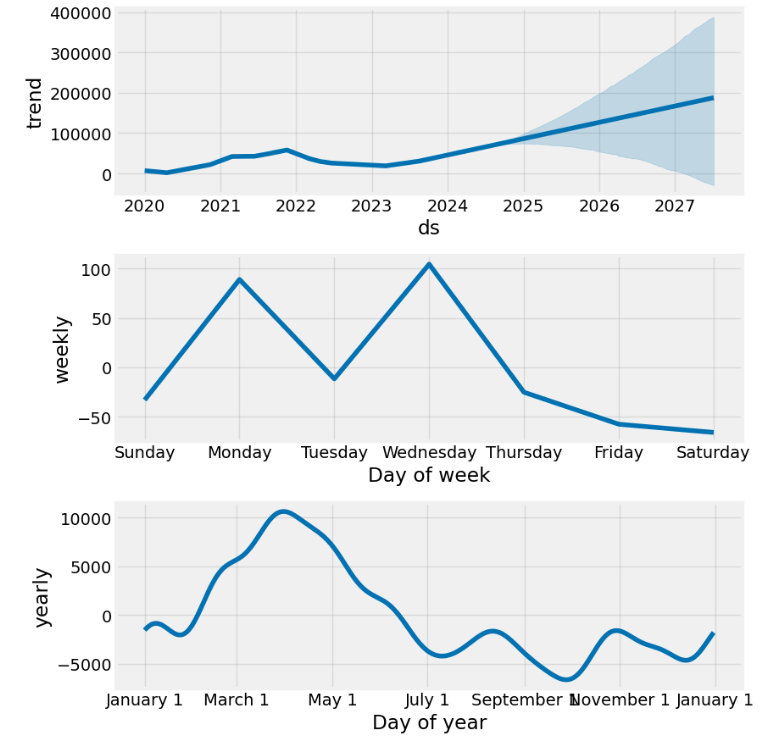
- Plotting the key components
model.plot_components(forecast);
- Plotting the original price vs forecast with confidence intervals
stock_price_forecast = forecast[['ds', 'yhat', 'yhat_lower', 'yhat_upper']]
df = pd.merge(stock_price, stock_price_forecast, on='ds', how='right')
df.set_index('ds').plot(figsize=(16,8), color=['royalblue', "#34495e", "#e74c3c", "#e74c3c"], grid=True);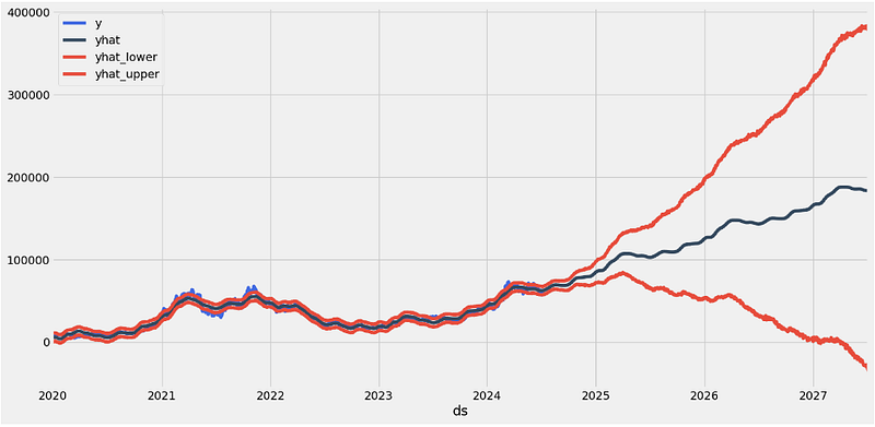
- Splitting the Date column into 3 parts (year/month/day) and fitting the Prophet model
stock_price['dayname'] = stock_price['ds'].dt.day_name()
stock_price['month'] = stock_price['ds'].dt.month
stock_price['year'] = stock_price['ds'].dt.year
stock_price['month/year'] = stock_price['month'].map(str) + '/' + stock_price['year'].map(str)

stock_price = pd.merge(stock_price,
                       stock_price['month/year'].drop_duplicates().reset_index(drop=True).reset_index(),
                       on='month/year',
                       how='left')

stock_price = stock_price.rename(columns={'index':'month/year_index'})

loop_list = stock_price['month/year'].unique().tolist()
max_num = len(loop_list) - 1
forecast_frames = []

for num, item in enumerate(loop_list):

    if  num == max_num:
        pass
    else:
        df = stock_price.set_index('ds')[
             stock_price[stock_price['month/year'] == loop_list[0]]['ds'].min():\
             stock_price[stock_price['month/year'] == item]['ds'].max()]

        df = df.reset_index()[['ds', 'y']]

        model = Prophet()
        model.fit(df)

        future = stock_price[stock_price['month/year_index'] == (num + 1)][['ds']]

        forecast = model.predict(future)
forecast_frames.append(forecast)- Plotting the in-sample forecast vs original price
stock_price_forecast = reduce(lambda top, bottom: pd.concat([top, bottom], sort=False), forecast_frames)
stock_price_forecast = stock_price_forecast[['ds', 'yhat', 'yhat_lower', 'yhat_upper']]

df = pd.merge(stock_price[['ds','y', 'month/year_index']], stock_price_forecast, on='ds')
df['Percent Change'] = df['y'].pct_change()
df.set_index('ds')[['y', 'yhat', 'yhat_lower', 'yhat_upper']].plot(figsize=(16,8), color=['royalblue', "#34495e", "#e74c3c", "#e74c3c"], grid=True)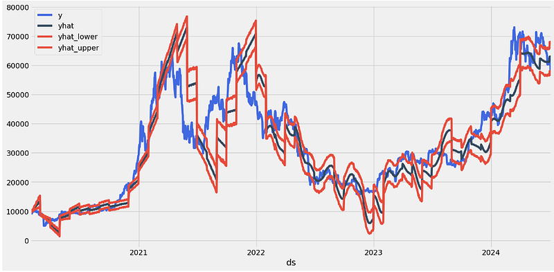
- Running cross-validation QC
from prophet.diagnostics import performance_metrics
df_p = performance_metrics(df_cv)
df_p.head()

  horizon  mse          rmse      mae     mape mdape smape coverage
0 37 days 40,821,715.40 6,389.19 4,890.31 0.18 0.12 0.22 0.55
1 38 days 41,109,990.95 6,411.71 4,913.96 0.18 0.12 0.22 0.55
2 39 days 41,311,288.83 6,427.39 4,922.43 0.19 0.12 0.22 0.55
3 40 days 41,641,137.72 6,452.99 4,943.99 0.19 0.12 0.22 0.55
4 41 days 42,299,834.63 6,503.83 5,003.53 0.19 0.12 0.23 0.54

from prophet.plot import plot_cross_validation_metric
fig = plot_cross_validation_metric(df_cv, metric='rmse')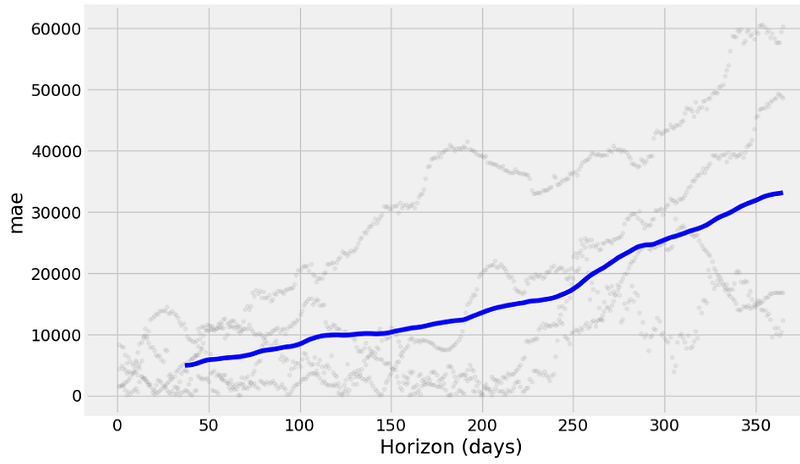
- Plotting MAPE
fig = plot_cross_validation_metric(df_cv, metric='mape')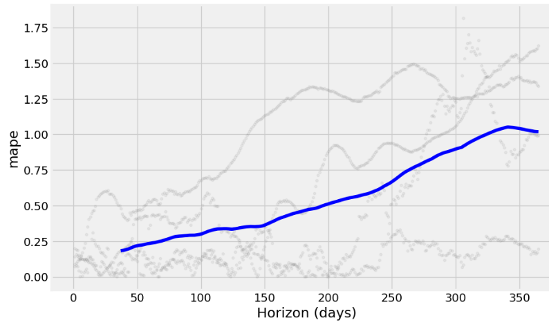
- Plotting MAE
fig = plot_cross_validation_metric(df_cv, metric='mae')- Implementing the Grid Search HPO and evaluating the model using MAE
# Define the hyperparameter grid
from sklearn.metrics import mean_absolute_error
param_grid = {
    'seasonality_mode': ['additive', 'multiplicative'],
    'changepoint_prior_scale': [0.01, 0.1, 1, 10],
    'seasonality_prior_scale': [0.01, 0.1, 1, 10],
}


# Helper function to evaluate the model
def evaluate_model(model, metric_func):
    df_cv = cross_validation(model, initial='1125 days', period='180 days', horizon='365 days')
    return metric_func(df_cv['y'], df_cv['yhat'])


# Grid search
best_params = {}
best_score = float('inf')

for mode in param_grid['seasonality_mode']:
    for cps in param_grid['changepoint_prior_scale']:
        for sps in param_grid['seasonality_prior_scale']:
            # Create a model with the current hyperparameters
            m = Prophet(seasonality_mode=mode, changepoint_prior_scale=cps, seasonality_prior_scale=sps)
            m.fit(stock_price)

            # Evaluate the model using Mean Absolute Error (MAE)
            score = evaluate_model(m, mean_absolute_error)

            # Update best parameters if necessary
            if score < best_score:
                best_score = score
                best_params = {
                    'seasonality_mode': mode,
                    'changepoint_prior_scale': cps,
                    'seasonality_prior_scale': sps
                }

print(best_params)


{'seasonality_mode': 'additive', 'changepoint_prior_scale': 0.1, 'seasonality_prior_scale': 10}

print(best_score)
8675.430008099349- Fitting the optimized model and creating the 1Y forecast
#Model with best parameters
m_best = Prophet(seasonality_mode= 'additive', changepoint_prior_scale = 0.1, seasonality_prior_scale = 10)
m_best.fit(stock_price)

#dataframe for the forecast(with 365 days)
future_best = m_best.make_future_dataframe(periods=365)
forecast_best = m_best.predict(future_best)

#plot the graph with the forecast data
fig1 = m.plot(forecast_best)
ax = fig1.gca()
ax.set_title("BTC-USD Stock Price Forecast", size=25)
ax.set_xlabel("Date", size=15)
ax.set_ylabel("Price", size=15)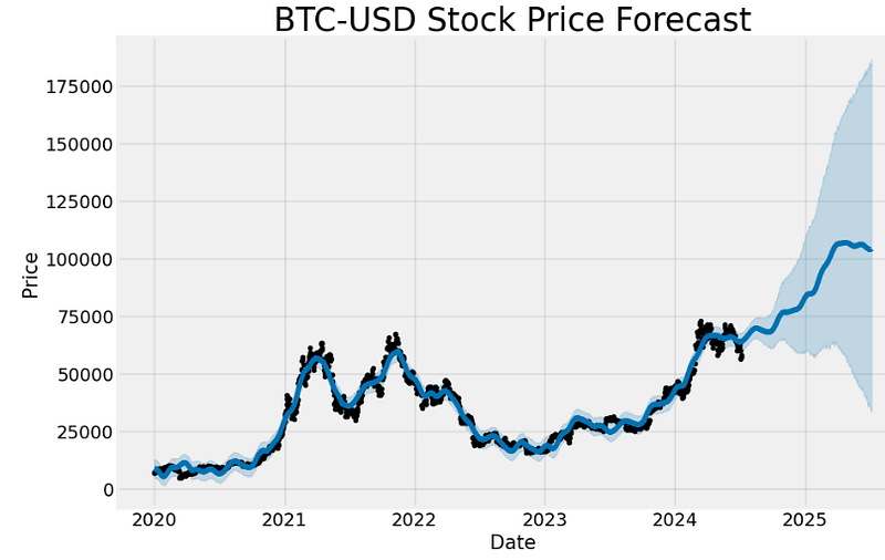
- Performing cross-validation QC with both scikit-learn and Prophet metrics
# Perform cross-validation
from sklearn.metrics import mean_squared_error
df_cv = cross_validation(m_best, initial='1125 days', period='180 days', horizon='365 days')

# Calculate performance metrics
df_metrics = performance_metrics(df_cv)

# Calculate MAE, MSE, and RMSE
mae = mean_absolute_error(df_cv['y'], df_cv['yhat'])
mse = mean_squared_error(df_cv['y'], df_cv['yhat'])
rmse = np.sqrt(mse)

print(f'Mean Absolute Error: {mae:.2f}')
print(f'Mean Squared Error: {mse:.2f}')
print(f'Root Mean Squared Error: {rmse:.2f}')

Mean Absolute Error: 8675.43
Mean Squared Error: 107375840.73
Root Mean Squared Error: 10362.23

from prophet.plot import plot_cross_validation_metric
df_cv = cross_validation(m_best, initial='1125 days', period='180 days', horizon='365 days')
fig = plot_cross_validation_metric(df_cv, metric='rmse')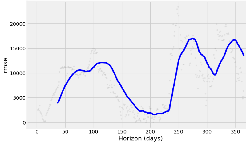
- Plotting MAPE
fig = plot_cross_validation_metric(df_cv, metric='mape')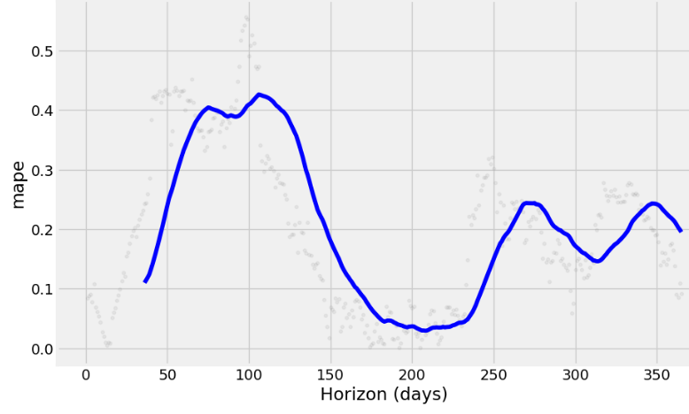
- Plotting MAE
fig = plot_cross_validation_metric(df_cv, metric='mae')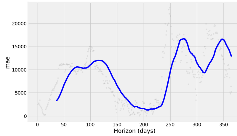
- Plotting both in-sample and out-of-sample 1Y Prophet forecasts with confidence intervals (original scale)
loop_list = stock_price['month/year'].unique().tolist()
max_num = len(loop_list) - 1
forecast_frames = []

for num, item in enumerate(loop_list):

    if  num == max_num:
        pass
    else:
        df = stock_price.set_index('ds')[
             stock_price[stock_price['month/year'] == loop_list[0]]['ds'].min():\
             stock_price[stock_price['month/year'] == item]['ds'].max()]

        df = df.reset_index()[['ds', 'y']]

        future = stock_price[stock_price['month/year_index'] == (num + 1)][['ds']]

        forecast = m_best.predict(future)
        forecast_frames.append(forecast)

stock_price_forecast1 = reduce(lambda top, bottom: pd.concat([top, bottom], sort=False), forecast_frames)
stock_price_forecast1 = stock_price_forecast1[['ds', 'yhat', 'yhat_lower', 'yhat_upper']]

df1 = pd.merge(stock_price[['ds','y', 'month/year_index']], stock_price_forecast1, on='ds')
df1['Percent Change'] = df1['y'].pct_change()
df1.set_index('ds')[['y', 'yhat', 'yhat_lower', 'yhat_upper']].plot(figsize=(16,8), color=['royalblue', "#34495e", "#e74c3c", "#e74c3c"], grid=True)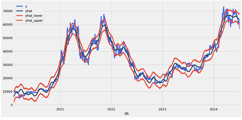
Modified Crypto Algo-Trading Strategies
- Let’s modify the Prophet-based crypto algo-trading strategies as follows
#Trading Algorithms
df=df1.copy()
df['Hold'] = (df['Percent Change'] + 1).cumprod()
df['Prophet'] = ((df['yhat'].shift(-1) > df['yhat']).shift(1) * (df['Percent Change']) + 1).cumprod()
df['Prophet Thresh']  = ((df['y'] < df['yhat_upper']).shift(1)* (df['Percent Change']) + 1).cumprod()
df['Seasonality'] = ((~df['ds'].dt.month.isin([8,9])).shift(1) * (df['Percent Change']) + 1).cumprod()

(df.dropna().set_index('ds')[['Hold', 'Prophet', 'Prophet Thresh','Seasonality']] * 1000).plot(figsize=(16,8), grid=True)

print(f"Hold = {df['Hold'].iloc[-1]*1000:,.0f}")
print(f"Prophet = {df['Prophet'].iloc[-1]*1000:,.0f}")
print(f"Prophet Thresh = {df['Prophet Thresh'].iloc[-1]*1000:,.0f}")
print(f"Seasonality = {df['Seasonality'].iloc[-1]*1000:,.0f}")

Hold = 6,090
Prophet = 87,595
Prophet Thresh = 18,681
Seasonality = 7,172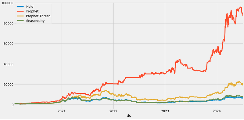
- Here, we have replaced the Prophet Thresh df[‘y’] > df[‘yhat_lower’] with the condition df[‘y’] < df[‘yhat_upper’] to get higher expected returns.
- Let’s optimize the above Prophet threshold
performance = {}

for x in np.linspace(.9,.99,10):
    y = ((df['y'] < df['yhat_upper']*x).shift(1)* (df['Percent Change']) + 1).cumprod()
    performance[x] = y

best_yhat = pd.DataFrame(performance).max().idxmax()
pd.DataFrame(performance).plot(figsize=(16,8), grid=True);
f'Best Yhat = {best_yhat:,.2f}'

'Best Yhat = 0.92'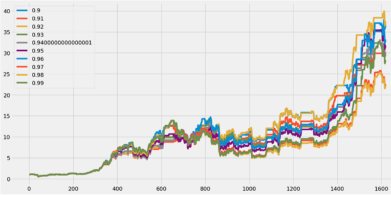
- Running backtesting with the Best Yhat = 0.92
df['Optimized Prophet Thresh']  = ((df['y'] < df['yhat_upper'] * best_yhat).shift(1) *
                                   (df['Percent Change']) + 1).cumprod()

(df.dropna().set_index('ds')[['Hold', 'Prophet', 'Prophet Thresh',
                              'Seasonality', 'Optimized Prophet Thresh']] * 1000).plot(figsize=(16,8), grid=True)

print(f"Hold = {df['Hold'].iloc[-1]*1000:,.0f}")
print(f"Prophet = {df['Prophet'].iloc[-1]*1000:,.0f}")
print(f"Prophet Thresh = {df['Prophet Thresh'].iloc[-1]*1000:,.0f}")
print(f"Seasonality = {df['Seasonality'].iloc[-1]*1000:,.0f}")
print(f"Optimized Prophet Thresh = {df['Optimized Prophet Thresh'].iloc[-1]*1000:,.0f}")

Hold = 6,090
Prophet = 87,595
Prophet Thresh = 18,681
Seasonality = 7,172
Optimized Prophet Thresh = 36,769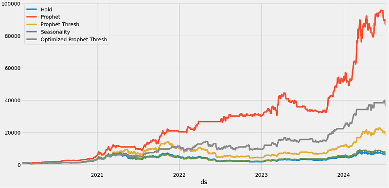
- Inferences:
- ROI(Prophet)/ROI(Optimized Prophet Thresh) ~ 2.4
- ROI(Prophet)/ROI(Hold) ~ 14.0
- ROI(Optimized Prophet Thresh)/ROI(Prophet Thresh) ~ 2.0
- ROI(Prophet Thresh)/ROI(Seasonality) ~ 2.5
- ROI(Seasonality)/ROI(Hold) ~ 1.0
Prophet Plotly Visualization with Change Points
- Let’s look at the available Prophet Plotly visualization options
mydf=stock_price[['ds','y']]
mm = Prophet()
mm.fit(mydf)
future = mm.make_future_dataframe(periods=365)
forecast = mm.predict(future)
from prophet.plot import plot_plotly

plot_plotly(mm, forecast)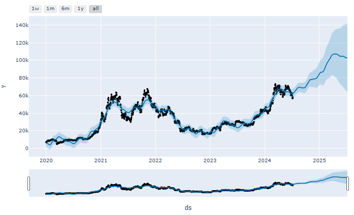
- Using Plotly to plot the Prophet forecast with change points
from prophet.plot import plot_plotly

plot_plotly(mm, forecast, changepoints=True)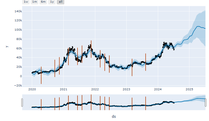
Conclusions
- In this post, we have analyzed ease-of-use Prophet (Facebook’s library for time series forecasting) to predict BTC-USD prices.
- We have used Yahoo Finance Python to download 2 datasets: (1) 730 days until 2024–07–06; (2) from 2020–01–01 to 2024–07–07.
- We have invoked dataset 1 to test the Box-Cox transformation and HPO with US holidays.
- We have downloaded dataset 2 to demonstrate the value of handling multiple seasonality by creating Prophet HPO forecasts in a loop after splitting the date ds column into 3 parts (year, month, and day).
- We have delved into details of Prophet cross-validation functionality by comparing several key metrics such as RMSE, MAPE, and MAE for both datasets.
- Dataset 2: final in-sample Prophet error metrics are as follows
Mean Absolute Error: 8675.43
Mean Squared Error: 107375840.73
Root Mean Squared Error: 10362.23- Dataset 2: the out-of-sample Prophet HPO error metrics for 350 horizon days yield
MAPE ~ 0.2-0.4, (MAE, RMSE) ~ 10k-15k- We have illustrated the value of using Plotly to plot Prophet forecasts with change points.
- Finally, we have used dataset 2 to explore several useful Prophet-based backtesting crypto algo-trading strategies against Hold benchmark.
- Backtesting results have shown that ROI(Prophet)/ROI(Hold) ~ 14.0.
- Our test confirm that Prophet trends can be correctly estimated without any external data. Because our time series have strong seasonal business cycles, we found that Prophet works quite well.
- One of the key advantages of Prophet over other statistical models and ML is its interpretability. Prophet offers a good baseline quickly, as you don’t have to craft time features.
- Overall, we conclude that a native handling of trend and seasonality features, that makes Prophet a good baseline model if the time series follows business cycles (cf. Resources).
References
- Share Price Forecasting Using Facebook Prophet
- Prophet Diagnostics
- Getting started with Facebook Prophet
- Time-Series Forecasting With Facebook Prophet
- BTC Price Prediction using FB Prophet
Contacts
Disclaimer
- The following disclaimer clarifies that the information provided in this article is for educational use only and should not be considered financial or investment advice.
- The information provided does not take into account your individual financial situation, objectives, or risk tolerance.
- Any investment decisions or actions you undertake are solely your responsibility.
- You should independently evaluate the suitability of any investment based on your financial objectives, risk tolerance, and investment timeframe.
- It is recommended to seek advice from a certified financial professional who can provide personalized guidance tailored to your specific needs.
- The tools, data, content, and information offered are impersonal and not customized to meet the investment needs of any individual. As such, the tools, data, content, and information are provided solely for informational and educational purposes only.
Resources
https://www.kaggle.com/code/alexkaggle95/stock-prices-forecast-plotly-prophet bad
https://www.kaggle.com/code/ghazanfarali/stock-price-analysis-and-forecasting var


