NVDA vs BTC Algorithmic Trading: Backtest BB, MACD & AO Trading Strategies

Comparing NVIDIA vs BTC-USD Historical Returns (Backtesting) using Bollinger Bands (BB), MACD & Awesome Oscillator (AO) Trading Strategies — it It About to Flip?

“Never depend on a single income. Make an investment to create a second source.” — Warren Buffett

Crypto News July 31, 2024: Since late 2022, NVDA’s stock has become a key indicator for both equity and crypto markets. The correlation between NVDA’s stock and BTC is strong; according to a source, the 3-month correlation between BTC and Nvidia is 0.71. Surprisingly, both hit bottom in late 2022 and have shown similar trends.
In this post, we will backtest NVDIA and BTC trading strategies: starting from fetching stock data, computing technical indicators, generating trading signals and finally comparing expected returns.
Firstly, we will compute the Bollinger Bands (BB) [1, 2] to identify the over-sold and over-bought signals of the NVDIA stock since 2022. While every strategy has its drawbacks, BB are among the most useful and commonly used tools in spotlighting extreme short-term security prices. Read more here.
Secondly, we will download the BTC-USD prices from Kraken’s API and build trading strategies based on the Moving Average Convergence/Divergence (MACD) and the Awesome Oscillator (AO) [3].
One of the biggest advantages of the MACD is that it’s both a trend and momentum indicator. It is designed to help investors identify price trends, measure trend momentum, and identify acceleration points to fine-tune market entry timing.
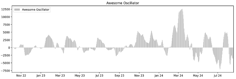
One of the key benefits of using the AO is its simplicity. The AO indicator provides traders with a clear and straightforward way to analyze market trends, as positive values indicate an uptrend and negative values indicate a downtrend.

Business Goals:

NVDA or BTC — What’s a better investment?
Given MicroStrategy’s success, what if NVDA were to adopt a similar BTC strategy?

Basic Imports & Settings

Importing and installing the necessary Python libraries

!pip install requests_html, yfinance, ccxt,ta, quantstats

import pandas as pd
import numpy as np
import yfinance as yf
import yahoo_fin.stock_info as si
import matplotlib.pyplot as plt
import matplotlib.dates as mdates
import ccxt
import ta
import quantstats as qs

V.i. more imports and settings on a as-needed basis.

Reading NVDA Close Price

Using Yahoo Finance to download the NVDA historical stock data

def load_data(tickers):
    data = pd.DataFrame(columns = tickers)
    for ticker in tickers:
        data[ticker] = yf.download(ticker, start_date)['Close']
        
    return data

tickers = ['NVDA']
start_date = '2020-01-01'

df = load_data(tickers)

df.tail()

NVDA
Date 
2024-08-13 116.139999
2024-08-14 118.080002
2024-08-15 122.860001
2024-08-16 124.580002
2024-08-19 130.000000

Plotting the NVDA Close price

fig, ax = plt.subplots(figsize=(12,6))
plt.title(f'Close Price - {tickers[0]}')
plt.ylabel('Price in USD')
plt.xlabel('Dates')
ax.plot(df['NVDA'], label = 'Close Price', alpha = 1., color = 'r')
plt.grid()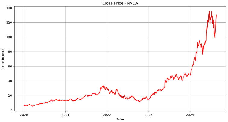

Bollinger Bands (BB)

Introducing the FinTa-style moving average functions EMA and DEMA

def EMA(ohlc,period = 9,column = "NVDA", adjust = True):
        """
        Exponential Weighted Moving Average - Like all moving average indicators, they are much better suited for trending markets.
        When the market is in a strong and sustained uptrend, the EMA indicator line will also show an uptrend and vice-versa for a down trend.
        EMAs are commonly used in conjunction with other indicators to confirm significant market moves and to gauge their validity.
        """

        return pd.Series(
            ohlc[column].ewm(span=period, adjust=adjust).mean(),
            name="{0} period EMA".format(period),
        )

def DEMA(ohlc,period = 9,column = "NVDA",adjust = True):
        """
        Double Exponential Moving Average - attempts to remove the inherent lag associated to Moving Averages
         by placing more weight on recent values. The name suggests this is achieved by applying a double exponential
        smoothing which is not the case. The name double comes from the fact that the value of an EMA (Exponential Moving Average) is doubled.
        To keep it in line with the actual data and to remove the lag the value 'EMA of EMA' is subtracted from the previously doubled EMA.
        Because EMA(EMA) is used in the calculation, DEMA needs 2 * period -1 samples to start producing values in contrast to the period
        samples needed by a regular EMA
        """

        DEMA = (
            2 * EMA(ohlc, period)
            - EMA(ohlc, period).ewm(span=period, adjust=adjust).mean()
        )

        return pd.Series(DEMA, name="{0} period DEMA".format(period))

Computing the Bollinger Bands (BB) [1, 2] in terms of the above two functions

sma=DEMA(df, period=30, column="NVDA",adjust=True).dropna()
rstd = df.rolling(window=30).std().dropna()

upper_band = sma + 2 * rstd['NVDA']
lower_band = sma - 2 * rstd['NVDA']

column_names=["upper"]
upper_band1=pd.DataFrame(upper_band, columns=column_names)
column_names=["lower"]
lower_band1=pd.DataFrame(lower_band, columns=column_names)
df_bollinger_band = df.join(upper_band1).join(lower_band1)
df_bollinger_band = df_bollinger_band.dropna()
df_bollinger_band.tail()

           NVDA       upper      lower
Date   
2024-08-13 116.139999 130.763241 90.159861
2024-08-14 118.080002 131.440269 91.046983
2024-08-15 122.860001 132.424561 92.682191
2024-08-16 124.580002 133.754831 94.159677
2024-08-19 130.000000 135.858740 95.954941

Plotting the NVDA Close price & upper/lower BB

fig, ax = plt.subplots(figsize=(12,6))
ax.plot(df_bollinger_band['upper'], label = 'Upper Band', alpha = 1, 
               color = 'red')
ax.plot(df_bollinger_band['lower'], label = 'Lower Band', alpha = 1, 
               color = 'blue')
plt.title(f'Bollinger Bands - {tickers[0]}')
plt.ylabel('Price in USD')
plt.xlabel('Dates')
ax.plot(df_bollinger_band['NVDA'], label = 'Close Price', alpha = 0.5, color = 'black')
plt.legend(loc='upper left')
plt.grid()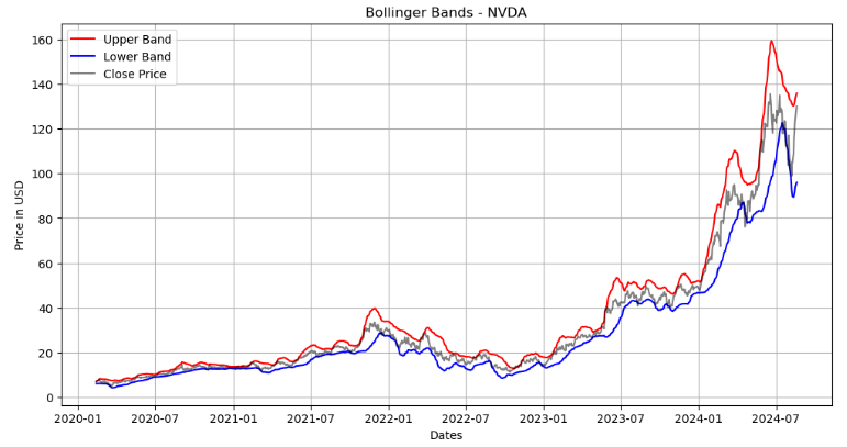

BB Trading Signals

Implementing the BB trading strategy as follows [1, 2]

buyers = df_bollinger_band[df_bollinger_band['NVDA'] <= df_bollinger_band['lower']]
sellers = df_bollinger_band[df_bollinger_band['NVDA'] >= df_bollinger_band['upper']]

def implement_bb_strategy(data,price='NVDA',upper='upper',lower='lower'):
    buy_price = []
    sell_price = []
    sma_signal = []
    signal = 0
    
    for i in range(len(data)):
        if data[price].iloc[i] > data[lower].iloc[i]:
            if signal != 1:
                buy_price.append(data[price].iloc[i])
                sell_price.append(np.nan)
                signal = 1
                sma_signal.append(signal)
            else:
                buy_price.append(np.nan)
                sell_price.append(np.nan)
                sma_signal.append(0)
        elif data[price].iloc[i] < data[upper].iloc[i]:
            if signal != -1:
                buy_price.append(np.nan)
                sell_price.append(data[price].iloc[i])
                signal = -1
                sma_signal.append(-1)
            else:
                buy_price.append(np.nan)
                sell_price.append(np.nan)
                sma_signal.append(0)
        else:
            buy_price.append(np.nan)
            sell_price.append(np.nan)
            sma_signal.append(0)
            
    return buy_price, sell_price, sma_signal

Plotting the BB strategy output

buy_price, sell_price, signal = implement_bb_strategy(df_bollinger_band)

plt.figure(figsize=(14,6))
plt.plot(df_bollinger_band['NVDA'], alpha = 0.8, label = 'NVDA')
plt.plot(df_bollinger_band['lower'], alpha = 0.6, label = 'BB LOWER')
plt.plot(df_bollinger_band['upper'], alpha = 0.6, label = 'BB UPPER')
plt.scatter(df_bollinger_band.index, buy_price, marker = '^', s = 100, color = 'darkblue', label = 'BUY SIGNAL')
plt.scatter(df_bollinger_band.index, sell_price, marker = 'v', s = 100, color = 'crimson', label = 'SELL SIGNAL')
plt.legend(loc = 'upper left')
plt.grid()
plt.title('NVDA BB TRADING SIGNALS')

NVDA BB Trading Signals: Output of implement_bb_strategy

Plotting the BB buyers & sellers

# Visualizing the Bolling Bands
fig, ax = plt.subplots(figsize=(12,6))
plt.title(f'Bollinger Band - {tickers[0]}')
plt.ylabel('Price in USD')
plt.xlabel('Dates')
ax.plot(df_bollinger_band['NVDA'], label = 'Close Price', alpha = 0.25, color = 'black')
ax.plot(df_bollinger_band['upper'], label = 'Upper Band', alpha = 0.25, color = 'red')
ax.plot(df_bollinger_band['lower'], label = 'Lower Band', alpha = 0.25, color = 'blue')
ax.fill_between(df_bollinger_band.index, df_bollinger_band['upper'], df_bollinger_band['lower'], color = '#F9E79F')
ax.scatter(buyers.index, buyers['NVDA'], label = 'Buy', alpha = 1, marker = '^', color = 'green')
ax.scatter(sellers.index, sellers['NVDA'], label = 'Sell', alpha = 1, marker = 'v', color = 'red')
plt.legend()
plt.grid()
plt.show()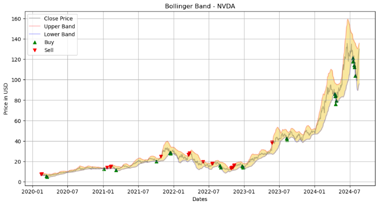

BB Strategy Returns

Creating the stock position

position = []
for i in range(len(signal)):
    if signal[i] > 1:
        position.append(0)
    else:
        position.append(1)
        
for i in range(len(df_bollinger_band['NVDA'])):
    if signal[i] == 1:
        position[i] = 1
    elif signal[i] == -1:
        position[i] = 0
    else:
        position[i] = position[i-1]

Plotting the NVDA daily returns: BB strategy vs Buy & Hold (B&H)

plt.figure(figsize=(12,6))
rets = df_bollinger_band['NVDA'].pct_change().dropna()
strat_rets = position[1:]*rets

plt.title('Daily Returns')
rets.plot(color = 'blue', alpha = 0.3, linewidth = 7,label='B&H Return')
strat_rets.plot(color = 'r', linewidth = 1,label='Strategy Return')
plt.legend()
plt.grid()
plt.show()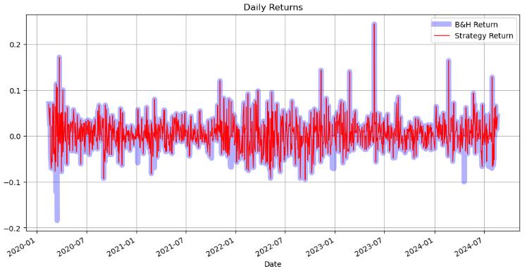

NVDA daily returns of the BB strategy vs Buy & Hold (B&H)

Plotting the NVDA cumulative returns: BB strategy vs B&H

rets_cum = (1 + rets).cumprod() - 1 
strat_cum = (1 + strat_rets).cumprod() - 1

plt.title('Cumulative Returns')
rets_cum.plot(color = 'blue', alpha = 0.3, linewidth = 7,label='B&H Return')
strat_cum.plot(color = 'r', linewidth = 2,label='Strategy Return')
plt.legend()
plt.grid(color='grey')
plt.show()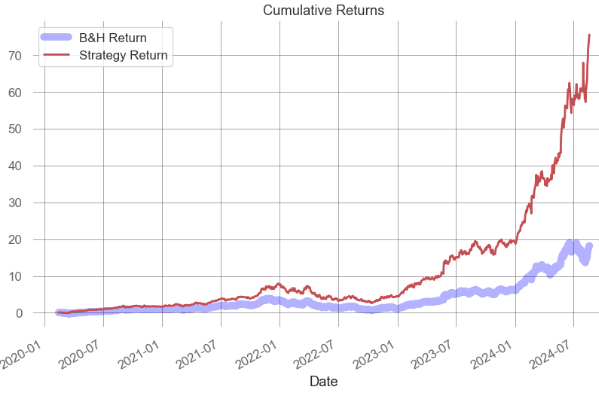

NVDA cumulative returns: BB strategy vs B&H

Reading BTC-USD Close Price

Using the Kraken API to read the BTC-USD stock historical data [3]

# Kraken API
exchange = ccxt.kraken()

# We define the symbol and timeframe
symbol = 'BTC/USD'
timeframe = '1d'

# We fetch OHLCV data
ohlcv = exchange.fetch_ohlcv(symbol, timeframe)

# We first convert to DataFrame then to Timestamp for a more readable format
df = pd.DataFrame(ohlcv, columns=['Timestamp', 'Open', 'High', 'Low', 'Close', 'Volume'])
df['Timestamp'] = pd.to_datetime(df['Timestamp'], unit='ms')
df.set_index('Timestamp', inplace=True)

# We now have our DataFrame
df

           Open    High    Low     Close   Volume
Timestamp     
2022-09-01 20049.4 20195.0 19560.0 20127.8 2829.586687
2022-09-02 20127.8 20434.9 19764.3 19954.6 3594.858626
2022-09-03 19954.0 20047.4 19655.6 19834.9 1409.931849
2022-09-04 19833.3 20010.0 19601.0 19995.8 1308.952671
2022-09-05 20000.0 20045.0 19642.9 19790.5 2418.522014
... ... ... ... ... ...
2024-08-16 57555.0 59800.0 57100.9 58898.4 1659.798395
2024-08-17 58895.6 59682.2 58812.4 59473.3 456.341715
2024-08-18 59473.4 60234.4 58451.6 58466.5 812.959316
2024-08-19 58466.5 59593.0 57860.8 59493.7 1313.020804
2024-08-20 59493.7 61391.9 59402.0 60682.2 952.381669
720 rows × 5 columns

MACD & AO Indicators

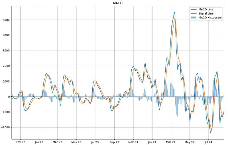
Calculating the MACD Line, Signal Line and Histogram [3]

# Calculate MACD Line, Signal Line and MACD Histogram
macd = ta.trend.MACD(df['Close'])

df['macd_line'] = macd.macd()  # MACD Line
df['macd_signal'] = macd.macd_signal()  # Signal Line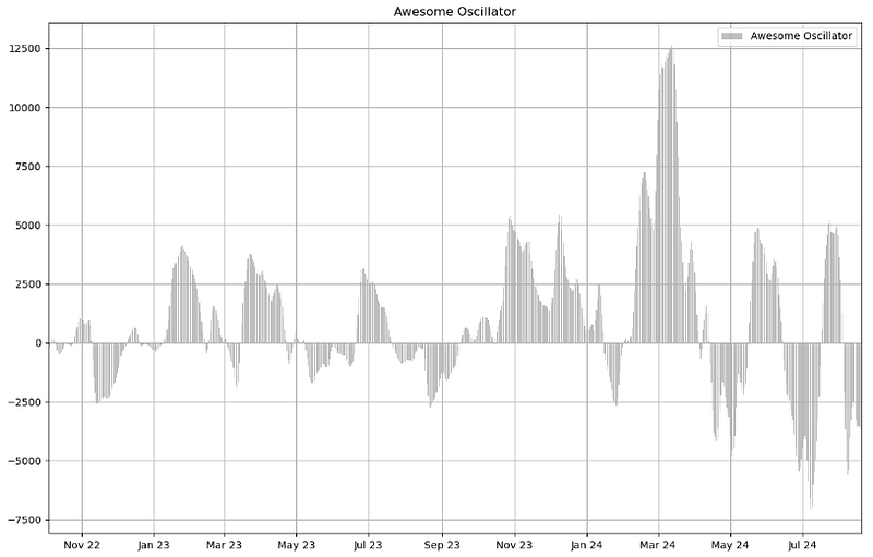
df['macd_hist'] = macd.macd_diff()  # MACD Histogram (MACD Line - Signal Line)

Calculating the Awesome Oscillator (AO)

# Calculate MACD Line, Signal Line and MACD Histogram
macd = ta.trend.MACD(df['Close'])

df['macd_line'] = macd.macd()  # MACD Line
df['macd_signal'] = macd.macd_signal()  # Signal Line
df['macd_hist'] = macd.macd_diff()  # MACD Histogram (MACD Line - Signal Line)

# Calculate Awesome Oscillator
ao = ta.momentum.AwesomeOscillatorIndicator(df['High'], df['Low'])

df['ao'] = ao.awesome_oscillator()  # Awesome Oscillator

df

           Open     High    Low    Close   Volume      macd_line macd_signal macd_hist ao
Timestamp         
2022-09-01 20049.4 20195.0 19560.0 20127.8 2829.586687 NaN NaN NaN NaN
2022-09-02 20127.8 20434.9 19764.3 19954.6 3594.858626 NaN NaN NaN NaN
2022-09-03 19954.0 20047.4 19655.6 19834.9 1409.931849 NaN NaN NaN NaN
2022-09-04 19833.3 20010.0 19601.0 19995.8 1308.952671 NaN NaN NaN NaN
2022-09-05 20000.0 20045.0 19642.9 19790.5 2418.522014 NaN NaN NaN NaN
... ... ... ... ... ... ... ... ... ...
2024-08-16 57555.0 59800.0 57100.9 58898.4 1659.798395 -1269.449533 -1161.663033 -107.786500 -3568.995588
2024-08-17 58895.6 59682.2 58812.4 59473.3 456.341715 -1177.388338 -1164.808094 -12.580244 -3523.468235
2024-08-18 59473.4 60234.4 58451.6 58466.5 812.959316 -1172.157619 -1166.277999 -5.879620 -3552.745588
2024-08-19 58466.5 59593.0 57860.8 59493.7 1313.020804 -1072.759676 -1147.574334 74.814659 -3681.345294
2024-08-20 59493.7 61391.9 59402.0 60682.2 952.381669 -887.849496 -1095.629367 207.779871 -3067.566765
720 rows × 9 columns

Dropping the NaN values

# Drop NaN values
df.dropna(inplace=True)
df.info()

<class 'pandas.core.frame.DataFrame'>
DatetimeIndex: 687 entries, 2022-10-04 to 2024-08-20
Data columns (total 9 columns):
 #   Column       Non-Null Count  Dtype  
---  ------       --------------  -----  
 0   Open         687 non-null    float64
 1   High         687 non-null    float64
 2   Low          687 non-null    float64
 3   Close        687 non-null    float64
 4   Volume       687 non-null    float64
 5   macd_line    687 non-null    float64
 6   macd_signal  687 non-null    float64
 7   macd_hist    687 non-null    float64
 8   ao           687 non-null    float64
dtypes: float64(9)
memory usage: 53.7 KB

Plotting the BTC-USD Close price, the MACD and AO indicators

fig, ax = plt.subplots(3, figsize=(12,12), dpi=200)

# Plot BTC prices
ax[0].plot(df.index, df['Close'], label='BTC/USD')
ax[0].set_title('BTC/USD Prices - Last 687 days')
ax[0].legend(loc='upper left')
ax[0].set_xlim([df.index.min(), df.index.max()])
#ax[0].grid()

# Plot MACD Line, Signal Line and Histogram
ax[1].plot(df.index, df['macd_line'], label='MACD Line') # Plot MACD Line and Signal Line
ax[1].plot(df.index, df['macd_signal'], label='Signal Line') # Plot MACD Line and Signal Line
ax[1].bar(df.index, df['macd_hist'], alpha=0.5, label='MACD Histogram') # Plot MACD Histogram as bar plot
ax[1].set_title('MACD')
ax[1].legend(loc='upper left')
ax[1].set_xlim([df.index.min(), df.index.max()])
#ax[1].grid()

# Plot Awesome Oscillator
ax[2].bar(df.index, df['ao'], alpha=0.5, label='Awesome Oscillator', color='gray')
ax[2].set_title('Awesome Oscillator')
ax[2].legend(loc='upper left')
ax[2].set_xlim([df.index.min(), df.index.max()])
#ax[2].grid()

# Set date format
date_format = mdates.DateFormatter('%b %y')
ax[0].xaxis.set_major_formatter(date_format)
ax[1].xaxis.set_major_formatter(date_format)
ax[2].xaxis.set_major_formatter(date_format)

# Show the plot
plt.tight_layout()
plt.show()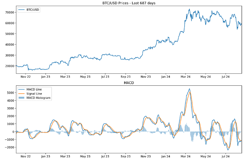

MACD/AO Trading Signals

Generating the buy/sell trading signals [3]

# Strategy 1
# Generating the buy "signal1"
df['signal1'] = np.where((df['macd_line'] > df['macd_signal']) & (df['ao'] > 0), 1, 0)
# Generating the "sell_signal1"
df['sell_signal1'] = np.where((df['macd_line'] < df['macd_signal']) & (df['ao'] < 0), 1, 0)

# Strategy 2
# Generating the buy "signal2" 
df['signal2'] = np.where((df['macd_line'] > df['macd_signal']) & (df['macd_line'].shift() < df['macd_signal'].shift()) & (df['ao'] > 0) & (df['ao'].shift() < 0), 1, 0)
# Generating the "sell_signal2"
df['sell_signal2'] = np.where((df['macd_line'] < df['macd_signal']) & (df['macd_line'].shift() > df['macd_signal'].shift()) & (df['ao'] < 0) & (df['ao'].shift() > 0), 1, 0)

# Counting the buy/sell signals
num_signals1 = df['signal1'].sum()
num_sells1 = df['sell_signal1'].sum()
num_signals2 = df['signal2'].sum()
num_sells2 = df['sell_signal2'].sum()

print(f"Number of buy signals in Strategy 1: {num_signals1}")
print(f"Number of sell signals in Strategy 1: {num_sells1}")
print(f"Number of buy signals in Strategy 2: {num_signals2}")
print(f"Number of sell signals in Strategy 2: {num_sells2}")

Number of buy signals in Strategy 1: 225
Number of sell signals in Strategy 1: 198
Number of buy signals in Strategy 2: 1
Number of sell signals in Strategy 2: 0

Plotting the buy/sell trading signals of Strategy 1 and a single buy signal of Strategy 2 to be neglected

fig, ax = plt.subplots(4, figsize=(12, 30))

# Plot ETH prices

ax[0].scatter(df[df['signal1'] == 1].index, df[df['signal1'] == 1]['Close'], color='g', marker='^', label='Buy Signal - Strategy 1')
ax[0].scatter(df[df['sell_signal1'] == 1].index, df[df['sell_signal1'] == 1]['Close'], color='r', marker='v', label='Sell Signal - Strategy 1')
ax[0].scatter(df[df['signal2'] == 1].index, df[df['signal2'] == 1]['Close'], color='b', marker='o', label='Buy Signal - Strategy 2', alpha=0.7)
#ax[0].scatter(df[df['sell_signal2'] == 1].index, df[df['sell_signal2'] == 1]['Close'], s=100,color='orange', marker='x', label='Sell Signal - Strategy 2', alpha=0.7)
ax[0].plot(df.index, df['Close'], label='BTC/USD',alpha=0.7)
ax[0].set_title('BTC/USD Prices - Last 687 days')
ax[0].legend()
ax[0].set_xlim([df.index.min(), df.index.max()])
ax[0].grid()

# Plot MACD Line, Signal Line and Histogram
ax[1].plot(df.index, df['macd_line'], label='MACD Line')
ax[1].plot(df.index, df['macd_signal'], label='Signal Line')
ax[1].bar(df.index, df['macd_hist'], alpha=0.5, label='MACD Histogram')
ax[1].set_title('MACD')
ax[1].legend()
ax[1].set_xlim([df.index.min(), df.index.max()])
ax[1].grid()

# Plot Awesome Oscillator
ax[2].bar(df.index, df['ao'], alpha=0.5, label='Awesome Oscillator', color='gray')
ax[2].set_title('Awesome Oscillator')
ax[2].legend()
ax[2].set_xlim([df.index.min(), df.index.max()])
ax[2].grid()

# Let's also set the appropriate date format
date_format = mdates.DateFormatter('%b %y')
for a in ax:
    a.xaxis.set_major_formatter(date_format)

# Plot
plt.tight_layout()
plt.show()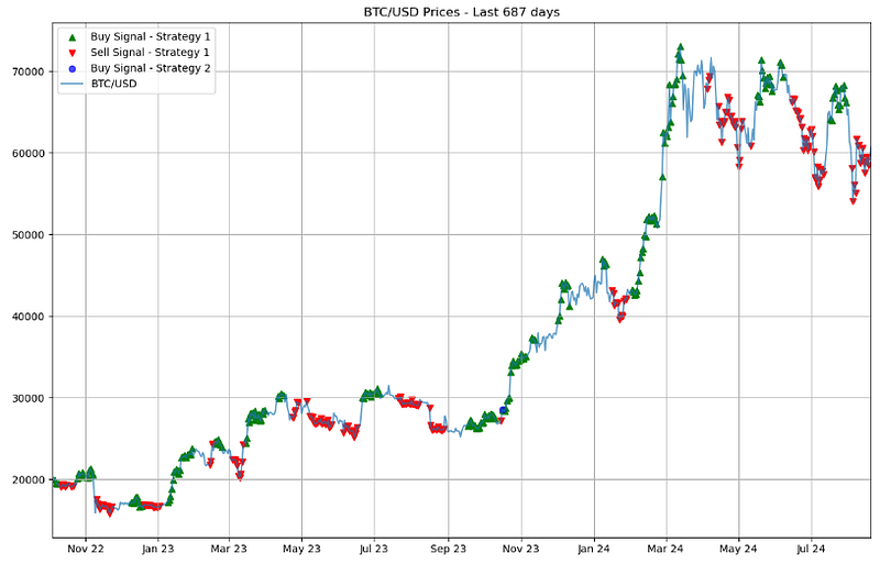

BTC-USD Close price vs buy/sell trading signals of Strategy 1

Plotting the MACD and AO indicators for the sake of comparison

MACD/AO Strategy Backtesting

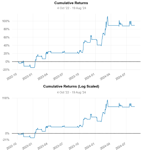
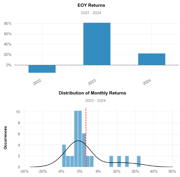
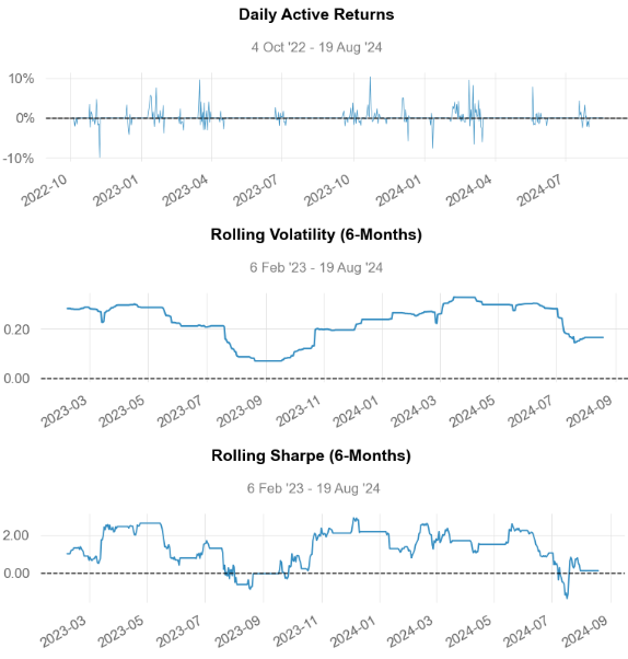
Using quantstats to backtest Strategy 1 [3]

# We calculate the daily returns
df['returns'] = df['Close'].pct_change()

# Strategy 1 returns
df['strategy1_returns'] = df['returns'] * df['signal1'].shift()
df['strategy1_cum_returns'] = (1 + df['strategy1_returns']).cumprod()

# Drop the NaN values
df.dropna(inplace=True)

# Let's print the report for Strategy 1
print("Strategy 1:")
qs.reports.full(df['strategy1_returns'])

Strategy 1:
Performance Metrics

Strategy
-------------------------  ----------
Start Period               2022-10-04
End Period                 2024-08-19
Risk-Free Rate             0.0%
Time in Market             33.0%

Cumulative Return          89.3%
CAGR﹪                     26.46%

Sharpe                     1.12
Prob. Sharpe Ratio         97.23%
Smart Sharpe               1.09
Sortino                    1.92
Smart Sortino              1.87
Sortino/√2                 1.36
Smart Sortino/√2           1.32
Omega                      1.44

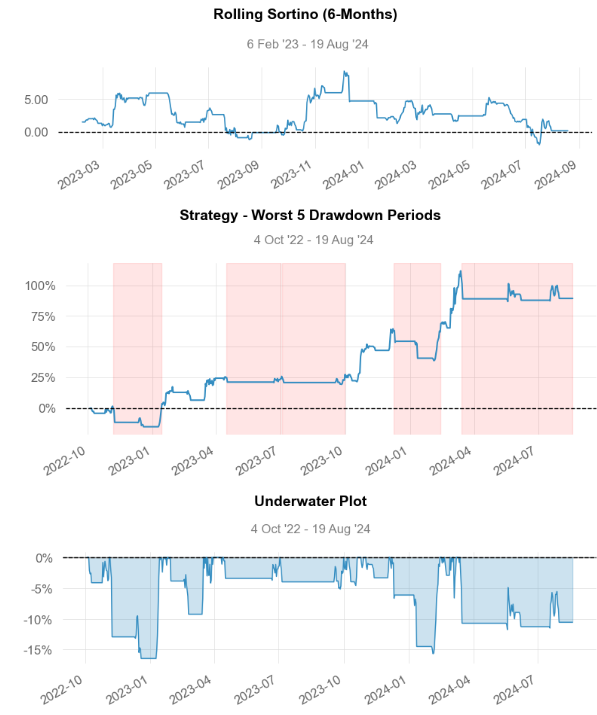
Max Drawdown               -16.44%
Longest DD Days            159
Volatility (ann.)          23.42%
Calmar                     1.61
Skew                       1.38
Kurtosis                   17.17

Expected Daily %           0.09%
Expected Monthly %         2.81%
Expected Yearly %          23.7%
Kelly Criterion            14.96%
Risk of Ruin               0.0%
Daily Value-at-Risk        -2.32%
Expected Shortfall (cVaR)  -2.32%

Max Consecutive Wins       8
Max Consecutive Losses     4
Gain/Pain Ratio            0.44
Gain/Pain (1M)             1.87

Payoff Ratio               1.51
Profit Factor              1.44
Common Sense Ratio         2.01
CPC Index                  1.06
Tail Ratio                 1.4
Outlier Win Ratio          12.87
Outlier Loss Ratio         2.31

MTD                        0.0%
3M                         0.36%
6M                         11.42%
YTD                        22.56%
1Y                         56.6%
3Y (ann.)                  26.46%
5Y (ann.)                  26.46%
10Y (ann.)                 26.46%
All-time (ann.)            26.46%

Best Day                   10.33%
Worst Day                  -9.97%
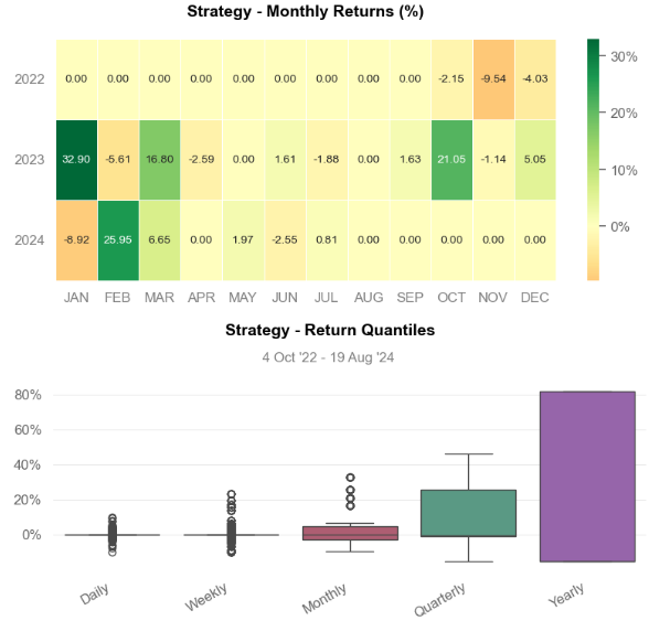
Best Month                 32.9%
Worst Month                -9.54%
Best Year                  81.81%
Worst Year                 -15.05%

Avg. Drawdown              -3.72%
Avg. Drawdown Days         22
Recovery Factor            4.33
Ulcer Index                0.08
Serenity Index             0.94

Avg. Up Month              11.44%
Avg. Down Month            -4.27%
Win Days %                 48.89%
Win Month %                52.63%
Win Quarter %              50.0%
Win Year %                 66.67%
None
Worst 5 Drawdowns
   Start     Valley     End       Days Max Drawdown 99% Max Drawdown
1 2022-11-06 2022-12-19 2023-01-13 69  -16.444587        -15.474868
2 2023-12-09 2024-02-04 2024-02-13 67  -15.678754        -15.562739
3 2024-03-14 2024-05-19 2024-08-19 159 -11.757961        -11.278155
4 2023-01-30 2023-02-24 2023-03-16 46  -9.249899         -6.713859
5 2024-03-05 2024-03-05 2024-03-07 3   -6.616796         -3.255414

Strategy 1 Visualization

Strategy EOY Returns & Distribution of Monthly Returns

Strategy Daily Active Returns, Rolling Volatility and Sharpe (6-Months)

Rolling Sortino (6-Months), Worst 5 Drawdown Periods, and Underwater Plot

Strategy Monthly Returns (%) and Return Quantiles

Conclusions

NVDA 4Y BB Strategy [1, 2] Cumulative Return is ~ 75% as compared to B&H Return of 20%.
BTC-USD 2Y MACD-based Strategy [3] Cumulative Return is ~ 89%, CAGR ~ 26%, Volatility (ann.) is 23.42%, the Kelly Criterion is 14.96%, CVaR is -2.32%, Sortino is 1.92 and Sharpe is 1.12.
Results indicate that NVDA will have no choice but to adopt BTC and integrate “digital gold” into its business processes as a valuable hedge against inflation.
Bottom Line: Holding NVDA stock and BTC together in a portfolio can reduce certain risks compared to keeping just one of them.

References

Explore More

Contacts

Disclaimer

The following disclaimer clarifies that the information provided in this article is for educational use only and should not be considered financial or investment advice.
The information provided does not take into account your individual financial situation, objectives, or risk tolerance.
Any investment decisions or actions you undertake are solely your responsibility.
You should independently evaluate the suitability of any investment based on your financial objectives, risk tolerance, and investment timeframe.
It is recommended to seek advice from a certified financial professional who can provide personalized guidance tailored to your specific needs.
The tools, data, content, and information offered are impersonal and not customized to meet the investment needs of any individual. As such, the tools, data, content, and information are provided solely for informational and educational purposes only.