
Resolving Bias-Variance Tradeoff in BTC-USD Price Prediction: Incorporating Technical Indicators into XGBoost Regression with Optuna Hyperparameter Optimization

- The objective of this article is to decipher the optimal model selection and the bias-variance tradeoff in BTC-USD price prediction using regression techniques.
- Bias-variance tradeoff denotes the (nonlinear) relationship between the complexity and sensitivity of a supervised Machine Learning (ML) model.
- In practice, optimizing ML feature selection while increasing the training dataset size is one of the most effective ways to address this challenge.
- Other solutions to address bias and variance issues include:
- Regularization techniques like L1 (Lasso) and L2 (Ridge) to mitigate overfitting.
- Cross-validation to assess ML model’s performance on different subsets of the data.
- Ensemble ML techniques such as Random Forests and Gradient Boosting that combine multiple models to achieve better performance.
- If ML models suffer from high bias (underfitting), acquiring more data can help trained models capture more complex patterns.
- In this study, various Technical Trading Indicators (TTI) will be incorporated into the feature engineering process to enhance model inputs. By feeding these TTI engineered features into the ML algorithms, our trained model will learn to recognize complex relationships within the stock data.
- The proposed hybrid TTI-ML method complements traditional technical analysis by capturing subtle market trends, potentially mitigating false signals inherent in conventional methods. Furthermore, ML’s capability to handle large datasets helps identify nuanced patterns that might elude human bias.
- Inspired by the recent highly encouraging studies, we’ll utilize XGBRegressor to predict future BTC-USD prices by considering TTI as model features. XGBoost is an efficient implementation of gradient boosting that can be used for regression predictive modeling. At the moment it’s the de facto standard algorithm for getting accurate results from predictive modeling with ML.
- In fact, XGBRegressor uses a tree-based learning algorithm to make predictions. It’s really powerful but also has a lot of hyperparameters that can be tuned to improve the model’s performance even more than with the default settings. Read more here.
- In this post, we’ll tune the hyperparameters of an XGBRegressor model with Optuna. Optuna is rapidly taking over from GridSearchCV and RandomizedSearchCV as the preferred method for hyperparameter tuning.
- It is worthwhile to mention some of the key advantages of using Optuna:
- Efficient Search Space Exploration
- Automated Pruning Strategies
- Flexible API
- Parallelization
- Visualization Tools
- Investors need to predict future prices to determine the potential risks and returns associated with the stocks, enabling them to make informed decisions on buying, holding, or selling the stocks.
- Understanding the factors that could influence its stock price can help in making strategic decisions such as issuing new shares, stock buyback programs, and investment in R&D.
- Stock prices can be reflective of the company’s health and, by extension, the health of the economy.
- Knowing future stock price trends helps in liquidity management for both investors and the company.
- BTC can be traded 365 days a year, 24 hours a day.
- BTC can act as a hedge against equities and currencies or commodities.
- BTC’s strong multifractality leads to the market being more inefficient than traditional equities.
Contents:
- Python Imports & Installations
- Reading & Analyzing the Input BTC-USD Stock Data
- Time-Zoomed Common FinTech Analysis of Stock Returns
- Plotting BTC-USD Candlesticks with basic Technical Indicators
- TTI-Based ML Feature Engineering
- Training & Testing XGBoost Regression Model
- Optuna XGBoost Model Hyperparameter Optimization
- Evaluation & Interpretation of the Final Optuna-XGBoost Model
Let’s delve into the specifics of the proposed methodology.
Basic Python Imports & Installations
- Setting the working directory YOURPATH, importing and installing Python libraries
import os
os.chdir('YOURPATH')    # Set working directory
os. getcwd()

#Installing Libraries

!pip install plotly, yfinance, ta, quantstats, sklearn, xgboost

# Importing Libraries

# Data Handling
import pandas as pd
import numpy as np

# Data Visualization
import matplotlib.pyplot as plt
import seaborn as sns
import plotly.express as px
import plotly.graph_objs as go
import matplotlib.ticker as mtick
from plotly.offline import init_notebook_mode
init_notebook_mode(connected=True)

# Financial Data Analysis
import yfinance as yf
import ta
import quantstats as qs

# Machine Learning
from sklearn.metrics import roc_auc_score, roc_curve, auc

# Models
from sklearn.linear_model import LogisticRegression
from xgboost import XGBClassifier
from lightgbm import LGBMClassifier
from catboost import CatBoostClassifier
from sklearn.ensemble import AdaBoostClassifier, RandomForestClassifier

# Linear Regression Model
from sklearn.linear_model import LinearRegression


# Hiding warnings
import warnings
warnings.filterwarnings("ignore")
Reading & Analyzing the Input BTC-USD Stock Data
- Loading the input BTC-USD stock data using Yahoo Finance
benchmark_ = ["BTC-USD"]

start_date_ = "2021-01-03"
end_date_  = "2024-06-08"

df = yf.download(benchmark_, start=start_date_, end=end_date_)
df.tail()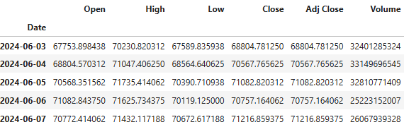
- Creating the Plotly candlestick chart for the above data (cf. tutorial)
# Creating the candlestick chart for BTC-USD
candlestick = go.Candlestick(x=df.index,
                open=df['Open'],
                high=df['High'],
                low=df['Low'],
                close=df['Adj Close'],
                increasing=dict(line=dict(color='black')),
                decreasing=dict(line=dict(color='red')),
                showlegend=False)

# Layout
layout = go.Layout(
    title='Adjusted BTC-USD Stock Price',
    yaxis=dict(title='Price (USD)'),
    xaxis=dict(title='Date'),
    template = 'ggplot2',
    xaxis_rangeslider_visible=False,
    yaxis_gridcolor='white',
    xaxis_gridcolor='white',
    yaxis_tickfont=dict(color='black'),
    xaxis_tickfont=dict(color='black'),
    margin=dict(t=50,l=50,r=50,b=50)
)

fig = go.Figure(data=[candlestick], layout=layout)

# Plotting annotation
fig.add_annotation(text='BTC-USD',
                    font=dict(color='gray', size=30),
                    xref='paper', yref='paper',
                    x=0.5, y=0.5,
                    showarrow=False,
                    opacity=1.0)


fig.show()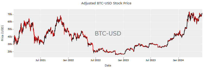
- Understanding the general structure of input data
# Inspect the index
print(df.index)
DatetimeIndex(['2021-01-03', '2021-01-04', '2021-01-05', '2021-01-06',
               '2021-01-07', '2021-01-08', '2021-01-09', '2021-01-10',
               '2021-01-11', '2021-01-12',
               ...
               '2024-05-29', '2024-05-30', '2024-05-31', '2024-06-01',
               '2024-06-02', '2024-06-03', '2024-06-04', '2024-06-05',
               '2024-06-06', '2024-06-07'],
              dtype='datetime64[ns]', name='Date', length=1252, freq=None)

#Checking the shape

df.shape
(1252, 6)

#General info

df.info()
<class 'pandas.core.frame.DataFrame'>
DatetimeIndex: 1252 entries, 2021-01-03 to 2024-06-07
Data columns (total 6 columns):
 #   Column     Non-Null Count  Dtype
---  ------     --------------  -----
 0   Open       1252 non-null   float64
 1   High       1252 non-null   float64
 2   Low        1252 non-null   float64
 3   Close      1252 non-null   float64
 4   Adj Close  1252 non-null   float64
 5   Volume     1252 non-null   int64
dtypes: float64(5), int64(1)
memory usage: 68.5 KB

#Descriptive statistics of Adj Close price

df['Adj Close'].describe().T
count     1252.000000
mean     37893.080243
std      14711.213854
min      15787.284180
25%      26335.864258
50%      36367.060547
75%      47247.533203
max      73083.500000
Name: Adj Close, dtype: float64- Plotting the Volume column
df['Volume'].plot(title="Volume")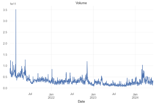
- Adding the column diff to the input DataFrame
df['diff'] = df.Open - df.Close
df['diff'].plot(title="BTC-USD Open-Close Price Difference")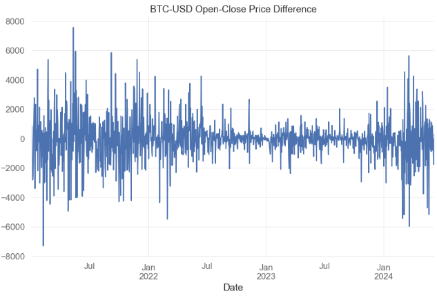
Time-Zoomed Common FinTech Analysis of Stock Returns
- Downloading the time-zoomed BTC-USD data
btc = qs.utils.download_returns('BTC-USD')
btc1 = btc.loc['2023-01-01':'2024-06-07']- Plotting the daily returns
print('\nBTC-USD Daily Returns Plot:\n')
qs.plots.daily_returns(btc1,benchmark='SPY')
BTC-USD Daily Returns Plot: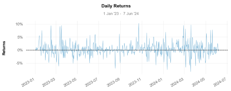
- Plotting the corresponding cumulative returns
print('\nBTC-USD Cumulative Returns Plot\n')
qs.plots.returns(btc1)

BTC-USD Cumulative Returns Plot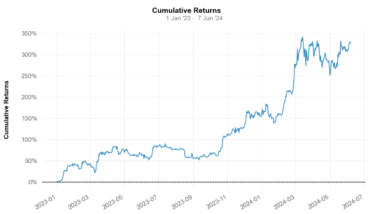
- Plotting the histogram of daily returns
print('\nBTC-USD Daily Returns Histogram')
qs.plots.histogram(btc1, resample = 'D')

BTC-USD Daily Returns Histogram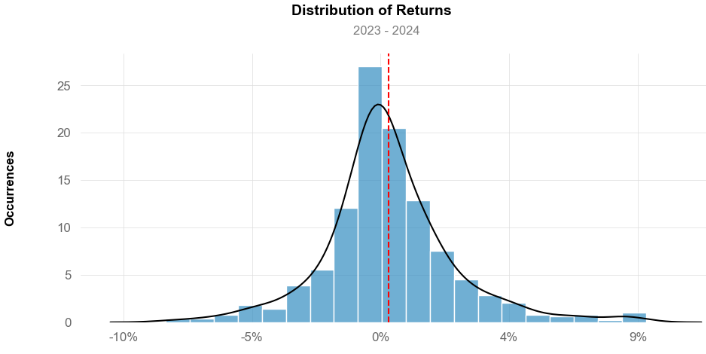
- Calculating the kurtosis, skewness, and std
print("BTC-USD's kurtosis: ", qs.stats.kurtosis(btc1).round(2))
TC-USD's kurtosis:  2.51

print("BTC-USD's skewness: ", qs.stats.skew(btc1).round(2))
BTC-USD's skewness:  0.57

print("BTC-USD's Standard Deviation: ", btc1.std())
BTC-USD's Standard Deviation: 0.025212506481976354- Calculating and plotting beta and alpha with respect to S&P 500
sp500 = qs.utils.download_returns('^GSPC')
sp500 = sp500.loc['2023-01-01':'2024-06-07']

btc2 = btc.loc['2023-01-03':'2024-06-06']
a=btc2.copy()
a_business_days = a[a.index.dayofweek < 5]

dfsp=sp500.to_frame()
dfbtc=btc2.to_frame()
dfspbtc = dfbtc.merge(dfsp, how='inner',right_index = True, left_index=True)

dfspbtc.info()

<class 'pandas.core.frame.DataFrame'>
DatetimeIndex: 359 entries, 2023-01-03 to 2024-06-06
Data columns (total 2 columns):
 #   Column   Non-Null Count  Dtype
---  ------   --------------  -----
 0   Close_x  359 non-null    float64
 1   Close_y  359 non-null    float64
dtypes: float64(2)
memory usage: 8.4 KB- Plotting the linear regression line with Close_y = S&P500 and Close_x = BTC-USD (daily returns)
sns.regplot(data=dfspbtc, x="Close_y", y="Close_x")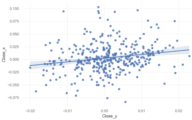
- Fitting the linear regression line
# Removing indexes
sp500_no_index = dfspbtc.Close_y.reset_index(drop = True)
a_business_days_no_index = dfspbtc.Close_x.reset_index(drop = True)

# Fitting linear relation among BTC-USD's returns and Benchmark
X = sp500_no_index.values.reshape(-1,1)
y = a_business_days_no_index.values.reshape(-1,1)
linreg = LinearRegression().fit(X, y)
beta = linreg.coef_[0]
alpha = linreg.intercept_
print('\n')
print('BTC-USD beta: ', beta.round(3))
print('\nBTC-USD alpha: ', alpha.round(3))

BTC-USD beta:  [0.721]

BTC-USD alpha: [0.002]- Calculating the Sharpe ratio
# Calculating Sharpe ratio
print("Sharpe Ratio for BTC-USD: ", qs.stats.sharpe(btc1).round(2))

Sharpe Ratio for BTC-USD:  1.95
Plotting BTC-USD Candlesticks with Basic Technical Indicators
- Plotting the BTC-USD Adj Close candlesticks with Volume and basic TTI such as EMA9, SMA(20, 50, 100, 200), Bollinger Bands (BB), RSI, and ATR
# Plotting Candlestick charts with indicators
from plotly.subplots import make_subplots
fig = make_subplots(rows=4, cols=1, shared_xaxes=True, vertical_spacing=0.05,row_heights=[0.6, 0.10, 0.10, 0.20])

# Candlestick
fig.add_trace(go.Candlestick(x=df.index,
                             open=df['Open'],
                             high=df['High'],
                             low=df['Low'],
                             close=df['Adj Close'],
                             name='BTC-USD'),
              row=1, col=1)

# Moving Averages
fig.add_trace(go.Scatter(x=df.index,
                         y=df['EMA9'],
                         mode='lines',
                         line=dict(color='#90EE90'),
                         name='EMA9'),
              row=1, col=1)

fig.add_trace(go.Scatter(x=df.index,
                         y=df['SMA20'],
                         mode='lines',
                         line=dict(color='yellow'),
                         name='SMA20'),
              row=1, col=1)

fig.add_trace(go.Scatter(x=df.index,
                         y=df['SMA50'],
                         mode='lines',
                         line=dict(color='orange'),
                         name='SMA50'),
              row=1, col=1)

fig.add_trace(go.Scatter(x=df.index,
                         y=df['SMA100'],
                         mode='lines',
                         line=dict(color='purple'),
                         name='SMA100'),
              row=1, col=1)

fig.add_trace(go.Scatter(x=df.index,
                         y=df['SMA200'],
                         mode='lines',
                         line=dict(color='red'),
                         name='SMA200'),
              row=1, col=1)

# Bollinger Bands
fig.add_trace(go.Scatter(x=df.index,
                         y=df['BB_UPPER'],
                         mode='lines',
                         line=dict(color='#00BFFF'),
                         name='Upper Band'),
              row=1, col=1)

fig.add_trace(go.Scatter(x=df.index,
                         y=df['BB_LOWER'],
                         mode='lines',
                         line=dict(color='#00BFFF'),
                         name='Lower Band'),
              row=1, col=1)

fig.add_annotation(text='BTC-USD',
                    font=dict(color='white', size=40),
                    xref='paper', yref='paper',
                    x=0.5, y=0.65,
                    showarrow=False,
                    opacity=0.2)


# Relative Strengh Index (RSI)
fig.add_trace(go.Scatter(x=df.index,
                         y=df['RSI'],
                         mode='lines',
                         line=dict(color='#CBC3E3'),
                         name='RSI'),
              row=2, col=1)

# Adding marking lines at 70 and 30 levels
fig.add_shape(type="line",
              x0=df.index[0], y0=70, x1=df.index[-1], y1=70,
              line=dict(color="red", width=2, dash="dot"),
              row=2, col=1)
fig.add_shape(type="line",
              x0=df.index[0], y0=30, x1=df.index[-1], y1=30,
              line=dict(color="#90EE90", width=2, dash="dot"),
              row=2, col=1)

# Average True Range (ATR)
fig.add_trace(go.Scatter(x=df.index,
                         y=df['ATR'],
                         mode='lines',
                         line=dict(color='#00BFFF'),
                         name='ATR'),
              row=3, col=1)


# Volume
fig.add_trace(go.Bar(x=df.index,
                     y=df['Volume'],
                     name='Volume',
                     marker=dict(color='orange', opacity=1.0)),
              row=4, col=1)


# Layout
fig.update_layout(title='BTC-USD Candlestick Chart & Indicators',
                  yaxis=dict(title='Price (USD)'),
                  height=1000,
                 template = 'plotly_dark')

# Axes and subplots
fig.update_xaxes(rangeslider_visible=False, row=1, col=1)
fig.update_xaxes(rangeslider_visible=False, row=4, col=1)
fig.update_yaxes(title_text='Price (USD)', row=1, col=1)
fig.update_yaxes(title_text='RSI', row=2, col=1)
fig.update_yaxes(title_text='ATR', row=3, col=1)
fig.update_yaxes(title_text='Volume', row=4, col=1)
fig.show()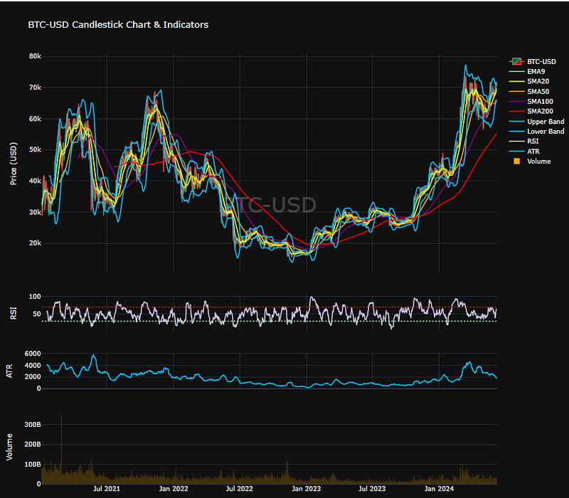
TTI-Based ML Feature Engineering
- Adapting the selected TTI functions from the FinTa library to our ML workflow
def TRIX(ohlc,period = 20,column = "Close",adjust = True):
        """
        The TRIX indicator calculates the rate of change of a triple exponential moving average.
        The values oscillate around zero. Buy/sell signals are generated when the TRIX crosses above/below zero.
        A (typically) 9 period exponential moving average of the TRIX can be used as a signal line.
        A buy/sell signals are generated when the TRIX crosses above/below the signal line and is also above/below zero.

        The TRIX was developed by Jack K. Hutson, publisher of Technical Analysis of Stocks & Commodities magazine,
        and was introduced in Volume 1, Number 5 of that magazine.
        """

        data = ohlc[column]

        def _ema(data, period, adjust):
            return pd.Series(data.ewm(span=period, adjust=adjust).mean())

        m = _ema(_ema(_ema(data, period, adjust), period, adjust), period, adjust)

        return pd.Series(100 * (m.diff() / m), name="{0} period TRIX".format(period))

def ER(ohlc, period = 10, column = "Close"):
        """The Kaufman Efficiency indicator is an oscillator indicator that oscillates between +100 and -100, where zero is the center point.
         +100 is upward forex trending market and -100 is downwards trending markets."""

        change = ohlc[column].diff(period).abs()
        volatility = ohlc[column].diff().abs().rolling(window=period).sum()

        return pd.Series(change / volatility, name="{0} period ER".format(period))

def TP(ohlc,open="Open",close="Close",high="High",low="Low"):
        """Typical Price refers to the arithmetic average of the high, low, and closing prices for a given period."""

        return pd.Series((ohlc[high] + ohlc[low] + ohlc[close]) / 3, name="TP")


def VWAP(ohlcv,colvol="Volume"):
        """
        The volume weighted average price (VWAP) is a trading benchmark used especially in pension plans.
        VWAP is calculated by adding up the dollars traded for every transaction (price multiplied by number of shares traded) and then dividing
        by the total shares traded for the day.
        """

        return pd.Series(
            ((ohlcv[colvol] * TP(ohlcv,open="Open",close="Close",high="High",low="Low")).cumsum()) / ohlcv[colvol].cumsum(),
            name="VWAP.",
        )

def PPO(ohlc,
        period_fast = 12,
        period_slow = 26,
        signal = 9,
        column = "Close",
        adjust = True):
        """
        Percentage Price Oscillator
        PPO, PPO Signal and PPO difference.
        As with MACD, the PPO reflects the convergence and divergence of two moving averages.
        While MACD measures the absolute difference between two moving averages, PPO makes this a relative value by dividing the difference by the slower moving average
        """

        EMA_fast = pd.Series(
            ohlc[column].ewm(ignore_na=False, span=period_fast, adjust=adjust).mean(),
            name="EMA_fast",
        )
        EMA_slow = pd.Series(
            ohlc[column].ewm(ignore_na=False, span=period_slow, adjust=adjust).mean(),
            name="EMA_slow",
        )
        PPO = pd.Series(((EMA_fast - EMA_slow) / EMA_slow) * 100, name="PPO")
        PPO_signal = pd.Series(
            PPO.ewm(ignore_na=False, span=signal, adjust=adjust).mean(), name="SIGNAL"
        )
        PPO_histo = pd.Series(PPO - PPO_signal, name="HISTO")

        return pd.concat([PPO, PPO_signal, PPO_histo], axis=1)

def VW_MACD(ohlcv,period_fast = 12,period_slow = 26,signal = 9,column = "Close", colvol = "Volume", adjust = True):
        """"Volume-Weighted MACD" is an indicator that shows how a volume-weighted moving average can be used to calculate moving average convergence/divergence (MACD).
        This technique was first used by Buff Dormeier, CMT, and has been written about since at least 2002."""

        vp = ohlcv[colvol] * ohlcv[column]
        _fast = pd.Series(
            (vp.ewm(ignore_na=False, span=period_fast, adjust=adjust).mean())
            / (
                ohlcv[colvol]
                .ewm(ignore_na=False, span=period_fast, adjust=adjust)
                .mean()
            ),
            name="_fast",
        )

        _slow = pd.Series(
            (vp.ewm(ignore_na=False, span=period_slow, adjust=adjust).mean())
            / (
                ohlcv[colvol]
                .ewm(ignore_na=False, span=period_slow, adjust=adjust)
                .mean()
            ),
            name="_slow",
        )

        MACD = pd.Series(_fast - _slow, name="MACD")
        MACD_signal = pd.Series(
            MACD.ewm(ignore_na=False, span=signal, adjust=adjust).mean(), name="SIGNAL"
        )

        return pd.concat([MACD, MACD_signal], axis=1)

def MOM(ohlc, period = 10, column = "Close"):
        """Market momentum is measured by continually taking price differences for a fixed time interval.
        To construct a 10-day momentum line, simply subtract the closing price 10 days ago from the last closing price.
        This positive or negative value is then plotted around a zero line."""

        return pd.Series(ohlc[column].diff(period), name="MOM".format(period))

def ROC(ohlc, period = 12, column = "Close"):
        """The Rate-of-Change (ROC) indicator, which is also referred to as simply Momentum,
        is a pure momentum oscillator that measures the percent change in price from one period to the next.
        The ROC calculation compares the current price with the price “n” periods ago."""

        return pd.Series(
            (ohlc[column].diff(period) / ohlc[column].shift(period)) * 100, name="ROC"
        )

def TR(ohlc,high="High",low="Low",close="Close"):
        """True Range is the maximum of three price ranges.
        Most recent period's high minus the most recent period's low.
        Absolute value of the most recent period's high minus the previous close.
        Absolute value of the most recent period's low minus the previous close."""

        TR1 = pd.Series(ohlc[high] - ohlc[low]).abs()  # True Range = High less Low

        TR2 = pd.Series(
            ohlc[high] - ohlc[close].shift()
        ).abs()  # True Range = High less Previous Close

        TR3 = pd.Series(
            ohlc[close].shift() - ohlc[low]
        ).abs()  # True Range = Previous Close less Low

        _TR = pd.concat([TR1, TR2, TR3], axis=1)

        _TR["TR"] = _TR.max(axis=1)

        return pd.Series(_TR["TR"], name="TR")

def ATR(ohlc, period = 14,high="High",low="Low",close="Close"):
        """Average True Range is moving average of True Range."""

        mytr=TR(ohlc,high=high,low=low,close=close)
        return pd.Series(
            mytr.rolling(center=False, window=period).mean(),
            name="{0} period ATR".format(period),
        )
def SAR(ohlc, af = 0.02, amax = 0.2,high="High",low="Low"):
        """SAR stands for “stop and reverse,” which is the actual indicator used in the system.
        SAR trails price as the trend extends over time. The indicator is below prices when prices are rising and above prices when prices are falling.
        In this regard, the indicator stops and reverses when the price trend reverses and breaks above or below the indicator."""
        high1, low1 = ohlc[high], ohlc[low]

        # Starting values
        sig0, xpt0, af0 = True, high1[0], af
        _sar = [low1[0] - (high1 - low1).std()]

        for i in range(1, len(ohlc)):
            sig1, xpt1, af1 = sig0, xpt0, af0

            lmin = min(low1[i - 1], low1[i])
            lmax = max(high1[i - 1], high1[i])

            if sig1:
                sig0 = low1[i] > _sar[-1]
                xpt0 = max(lmax, xpt1)
            else:
                sig0 = high1[i] >= _sar[-1]
                xpt0 = min(lmin, xpt1)

            if sig0 == sig1:
                sari = _sar[-1] + (xpt1 - _sar[-1]) * af1
                af0 = min(amax, af1 + af)

                if sig0:
                    af0 = af0 if xpt0 > xpt1 else af1
                    sari = min(sari, lmin)
                else:
                    af0 = af0 if xpt0 < xpt1 else af1
                    sari = max(sari, lmax)
            else:
                af0 = af
                sari = xpt0

            _sar.append(sari)

        return pd.Series(_sar, index=ohlc.index)

def DMI(ohlc, period = 14, adjust = True,high="High",low="Low",close="Close"):
        """The directional movement indicator (also known as the directional movement index - DMI) is a valuable tool
         for assessing price direction and strength. This indicator was created in 1978 by J. Welles Wilder, who also created the popular
         relative strength index. DMI tells you when to be long or short.
         It is especially useful for trend trading strategies because it differentiates between strong and weak trends,
         allowing the trader to enter only the strongest trends.
        source: https://www.tradingview.com/wiki/Directional_Movement_(DMI)#CALCULATION

        :period: Specifies the number of Periods used for DMI calculation
        """

        ohlc["up_move"] = ohlc[high].diff()
        ohlc["down_move"] = -ohlc[low].diff()

        # positive Dmi
        def _dmp(row):
            if row["up_move"] > row["down_move"] and row["up_move"] > 0:
                return row["up_move"]
            else:
                return 0

        # negative Dmi
        def _dmn(row):
            if row["down_move"] > row["up_move"] and row["down_move"] > 0:
                return row["down_move"]
            else:
                return 0

        ohlc["plus"] = ohlc.apply(_dmp, axis=1)
        ohlc["minus"] = ohlc.apply(_dmn, axis=1)

        diplus = pd.Series(
            100
            * (ohlc["plus"] / ATR(ohlc, period = period,high=high,low=low,close=close))
            .ewm(alpha=1 / period, adjust=adjust)
            .mean(),
            name="DI+",
        )
        diminus = pd.Series(
            100
            * (ohlc["minus"] / ATR(ohlc, period = period,high=high,low=low,close=close))
            .ewm(alpha=1 / period, adjust=adjust)
            .mean(),
            name="DI-",
        )

        return pd.concat([diplus, diminus], axis=1)

def ADX(ohlc, period = 14, adjust = True,high="High",low="Low",column="Close"):
        """The A.D.X. is 100 * smoothed moving average of absolute value (DMI +/-) divided by (DMI+ + DMI-). ADX does not indicate trend direction or momentum,
        only trend strength. Generally, A.D.X. readings below 20 indicate trend weakness,
        and readings above 40 indicate trend strength. An extremely strong trend is indicated by readings above 50"""

        dmi = DMI(ohlc, period = period, adjust = adjust,high=high,low=low,close=column)
        return pd.Series(
            100
            * (abs(dmi["DI+"] - dmi["DI-"]) / (dmi["DI+"] + dmi["DI-"]))
            .ewm(alpha=1 / period, adjust=adjust)
            .mean(),
            name="{0} period ADX.".format(period),
        )

def AO(ohlc, slow_period = 34, fast_period = 5,high="High",low="Low"):
        """'EMA',
        Awesome Oscillator is an indicator used to measure market momentum. AO calculates the difference of a 34 Period and 5 Period Simple Moving Averages.
        The Simple Moving Averages that are used are not calculated using closing price but rather each bar's midpoints.
        AO is generally used to affirm trends or to anticipate possible reversals. """

        slow = pd.Series(
            ((ohlc[high] + ohlc[low]) / 2).rolling(window=slow_period).mean(),
            name="slow_AO",
        )
        fast = pd.Series(
            ((ohlc[high] + ohlc[low]) / 2).rolling(window=fast_period).mean(),
            name="fast_AO",
        )

        return pd.Series(fast - slow, name="AO")

def ADL(ohlcv,colvol="Volume",column="Close",high="High",low="Low"):
        """The accumulation/distribution line was created by Marc Chaikin to determine the flow of money into or out of a security.
        It should not be confused with the advance/decline line. While their initials might be the same, these are entirely different indicators,
        and their uses are different as well. Whereas the advance/decline line can provide insight into market movements,
        the accumulation/distribution line is of use to traders looking to measure buy/sell pressure on a security or confirm the strength of a trend."""

        MFM = pd.Series(
            ((ohlcv[column] - ohlcv[low])
            - (ohlcv[high] - ohlcv[column])) / (ohlcv[high] - ohlcv[low]),
            name="MFM",
        )  # Money flow multiplier
        MFV = pd.Series(MFM * ohlcv[colvol], name="MFV")
        return MFV.cumsum()

def OBV(ohlcv, column = "Close",colvol="Volume"):
        """
        On Balance Volume (OBV) measures buying and selling pressure as a cumulative indicator that adds volume on up days and subtracts volume on down days.
        OBV was developed by Joe Granville and introduced in his 1963 book, Granville's New Key to Stock Market Profits.
        It was one of the first indicators to measure positive and negative volume flow.
        Chartists can look for divergences between OBV and price to predict price movements or use OBV to confirm price trends.

        source: https://en.wikipedia.org/wiki/On-balance_volume#The_formula

        :param pd.DataFrame ohlc: 'open, high, low, close' pandas DataFrame
        :return pd.Series: result is pandas.Series
        """

        ohlcv["OBV"] = np.nan

        neg_change = ohlcv[column] < ohlcv[column].shift(1)
        pos_change = ohlcv[column] >= ohlcv[column].shift(1)
        no_change = ohlcv[column] == ohlcv[column].shift(1)

        if pos_change.any():
            ohlcv.loc[pos_change, "OBV"] = ohlcv[colvol]
        if neg_change.any():
            ohlcv.loc[neg_change, "OBV"] = -ohlcv[colvol]
        if no_change.any():
            ohlcv.loc[no_change, "OBV"] = ohlcv["OBV"].shift(1)

        return pd.Series(ohlcv["OBV"].cumsum(), name="OBV")

def WOBV(ohlcv, column = "Close",colvol="Volume"):
        """
        Weighted OBV
        Can also be seen as an OBV indicator that takes the price differences into account.
        In a regular OBV, a high volume bar can make a huge difference,
        even if the price went up only 0.01, and it it goes down 0.01
        instead, that huge volume makes the OBV go down, even though
        hardly anything really happened.
        """

        wobv = pd.Series(ohlcv[colvol] * ohlcv[column].diff(), name="WOBV")
        return wobv.cumsum()

def CFI(ohlcv, column = "Close", colvol="Volume",adjust = True):
        """
        Cummulative Force Index.
        Adopted from  Elder's Force Index.
        """

        fi1 = pd.Series(ohlcv[colvol] * ohlcv[column].diff())
        cfi = pd.Series(
            fi1.ewm(ignore_na=False, min_periods=9, span=10, adjust=adjust).mean(),
            name="CFI",
        )

        return cfi.cumsum()

def CHANDELIER(ohlc,short_period = 22,long_period = 22,k = 3,high="High",low="Low"):
        """
        Chandelier Exit sets a trailing stop-loss based on the Average True Range (ATR).

        The indicator is designed to keep traders in a trend and prevent an early exit as long as the trend extends.

        Typically, the Chandelier Exit will be above prices during a downtrend and below prices during an uptrend.
        """

        l = pd.Series(
            ohlc[high].rolling(window=long_period).max() - ATR(ohlc, 22) * k,
            name="Long.",
        )
        s = pd.Series(
            ohlc[low].rolling(window=short_period).min() + ATR(ohlc, 22) * k,
            name="Short.",
        )

return pd.concat([s, l], axis=1)- Let’s load the input data and compute TTI using the above functions without importing FinTa
import pandas as pd
import numpy as np

import matplotlib.pyplot as plt
import seaborn as sns
sns.set_style('whitegrid')
plt.style.use("fivethirtyeight")
%matplotlib inline

# For reading stock data from yahoo


import yfinance as yf

# For time stamps
from datetime import datetime
from math import sqrt
from math import sqrt
from sklearn.metrics import mean_squared_error
from sklearn.preprocessing import MinMaxScaler

#ignore the warnings
import warnings
warnings.filterwarnings('ignore')

symbols = ['BTC-USD']
start_date = '2021-01-01'
end_date = '2024-06-08'

data = yf.download(symbols, start=start_date, end=end_date)
df=data.copy()
df.tail()

           Open         High         Low          Close        Adj Close     Volume
Date
2024-06-03 67753.898438 70230.820312 67589.835938 68804.781250 68804.781250 32401285324
2024-06-04 68804.570312 71047.406250 68564.640625 70567.765625 70567.765625 33149696545
2024-06-05 70568.351562 71735.414062 70390.710938 71082.820312 71082.820312 32810771409
2024-06-06 71082.843750 71625.734375 70119.125000 70757.164062 70757.164062 25223152007
2024-06-07 70772.414062 71907.828125 70672.617188 71316.078125 71316.078125 30640977920df[['Short', 'Long']]=CHANDELIER(data,short_period = 50,long_period = 100,k = 3,high="High",low="Low")
df['CFI']=CFI(data, column = "Close", colvol="Volume",adjust = True)
df['WOBV']=WOBV(data, column = "Close",colvol="Volume")
df['OBV']=OBV(data, column = "Close",colvol="Volume")
df['ADL']=ADL(data,colvol="Volume",column="Close",high="High",low="Low")
df['AO']=AO(data, slow_period = 34, fast_period = 5,high="High",low="Low")
df["ADX"]=ADX(data, period = 20, adjust = True,high="High",low="Low",column="Close")
df["SAR"]=SAR(data, af = 0.02, amax = 0.2,high="High",low="Low")
df['ATR20']=ATR(data, period = 20,high="High",low="Low",close="Close")
df['TR']=TR(data,high="High",low="Low",close="Close")
df["ROC20"]=ROC(data, period = 20, column = "Close")
df["MOM20"]=MOM(data, period = 20, column = "Close")
df[["VWMACD", "VWMACD_signal"]]=VW_MACD(data, period_fast = 12, period_slow = 26,signal = 9,column = "Close",colvol = "Volume",adjust = True)
df[["PPO", "PPO_signal","PPO_histo"]]=PPO(data, period_fast = 12, period_slow = 26,signal = 9,column = "Close",adjust = True)
df['VWAP']=VWAP(data,colvol="Volume")
df['TRIX20']=TRIX(data, period=20,column = "Close",adjust = True)
df['ER20']=ER(data, period=20,column = "Close")- We can add the simple moving averages by importing the ta library
import ta
df['sma5'] = ta.trend.sma_indicator(df['Adj Close'],window = 5)
df['sma10'] = ta.trend.sma_indicator(df['Adj Close'],window = 10)
df['sma15'] = ta.trend.sma_indicator(df['Adj Close'],window = 15)
df['sma20'] = ta.trend.sma_indicator(df['Adj Close'],window = 20)
df['sma30'] = ta.trend.sma_indicator(df['Adj Close'],window = 30)
df['sma50'] = ta.trend.sma_indicator(df['Adj Close'],window = 50)
df['sma80'] = ta.trend.sma_indicator(df['Adj Close'],window = 80)
df['sma100'] = ta.trend.sma_indicator(df['Adj Close'],window = 100)
df['sma200'] = ta.trend.sma_indicator(df['Adj Close'],window = 200)- Calculating a few popular indicators as follows
def calculate_sma(data, window):
    return data.rolling(window=window).mean()


def calculate_macd(data, short_window=12, long_window=26, signal_window=9):
    short_ema = data.ewm(span=short_window, adjust=False).mean()
    long_ema = data.ewm(span=long_window, adjust=False).mean()
    macd = short_ema - long_ema
    signal_line = macd.ewm(span=signal_window, adjust=False).mean()
    return macd, signal_line


def calculate_rsi(data, window=14):
    delta = data.diff(1)
    gain = (delta.where(delta > 0, 0)).rolling(window=window).mean()
    loss = (-delta.where(delta < 0, 0)).rolling(window=window).mean()
    rs = gain / loss
    rsi = 100 - (100 / (1 + rs))
    return rsi


def calculate_vroc(volume, window=14):
    vroc = ((volume.diff(window)) / volume.shift(window)) * 100
    return vroc


if __name__ == "__main__":

    df["sma50"] = calculate_sma(df["Close"], 50)
    df["sma200"] = calculate_sma(df["Close"], 200)
    df["macd"], df["signal"] = calculate_macd(df["Close"])
    df["rsi14"] = calculate_rsi(df["Close"])
    df["vroc14"] = calculate_vroc(df["Volume"])

    df.dropna(inplace=True)

df.tail()- Splitting the input data
# Select ratio 0.8 or 0.7
ratio = 0.8

total_rows = df.shape[0]
train_size = int(total_rows*ratio)

# Split data into test and train
train = df[0:train_size]
test = df[train_size:]- We can create various combinations of features and compare their importance by training either XGBoost or Random Forest (RF) regressors
features = [
    "Volume",
    "macd",
    "signal",
    "rsi14",
    "vroc14",
    "TRIX20",
    "ER20",
    "VWAP",
    "PPO",
    "ATR20",
    "SAR",
    "ADL",
    "OBV",
    "WOBV",
    "CFI",
    "Long",
    "Short"
]
#example of features- Implementing the (optional) example of RF regression with GridSearchCV tuning
param_grid = {
    "n_estimators": [50, 100, 200],
    "max_depth": [10, 20, 30, None],
    "min_samples_split": [2, 5, 10],
    "min_samples_leaf": [1, 2, 4],
    "bootstrap": [True, False],
}

rf = RandomForestRegressor(random_state=42)
grid_search = GridSearchCV(
    estimator=rf, param_grid=param_grid, cv=5, n_jobs=-1, verbose=2
)
grid_search.fit(X_train, y_train)

print(f"Best parameters: {grid_search.best_params_}")

best_rf = grid_search.best_estimator_
best_rf.fit(X_train, y_train)

Fitting 5 folds for each of 216 candidates, totalling 1080 fits
Best parameters: {'bootstrap': True, 'max_depth': 30, 'min_samples_leaf': 1, 'min_samples_split': 2, 'n_estimators': 200}

feature_importances = best_rf.feature_importances_
importance_df = pd.DataFrame(
    {"Feature": features, "Importance": feature_importances}
)

importance_df = importance_df.sort_values(by="Importance", ascending=False)

plt.figure(figsize=(10, 6))
sns.barplot(x="Importance", y="Feature", data=importance_df)
plt.title("Feature Importances of Technical Indicators")
plt.show()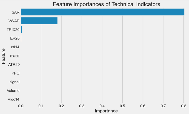
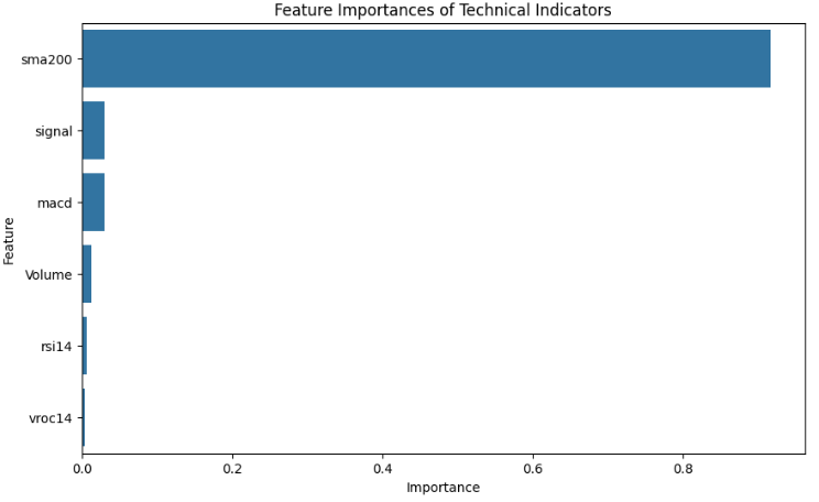
- Let’s consider another set of features
features = [
    "Volume",
    "macd",
    "sma200",
    "signal",
    "rsi14",
    "vroc14",
]
Training & Testing XGBoost Regression Model
- As an example, let’s consider the following features
features = [
    "sma5","sma10","sma15"
]- Defining the train/test features and target datasets
X_train = train[features]
y_train = train["Close"]

X_test = test[features]
y_test = test['Close']- Training and default XGBoost model
import xgboost as xgb

model = xgb.XGBRegressor(

)

model.fit(
    X_train,
    y_train,
    eval_set = [(X_train, y_train), (X_test, y_test)],
    early_stopping_rounds = 20,
    verbose = False
)- Checking the feature importance (for this example)
# Check feature importance
xgb.plot_importance(model, height=0.9)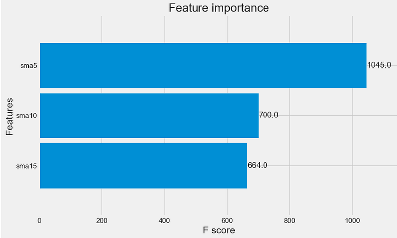
Optuna XGBoost Model Hyperparameter Optimization
- Selecting the following 11 features
features = [
    "Volume",
    "TRIX20",
    "ER20",
    "VWAP",
    "PPO",
    "ATR20",
    "SAR",
    "ADL",
    "OBV",
    "WOBV",
    "CFI",
    "Short"
]- Implementing the Optuna XGBoost hyperparameter optimization workflow
import xgboost as xgb
from sklearn.metrics import mean_squared_error
import optuna

def objective(trial):
    params = {
        "objective": "reg:squarederror",
        "n_estimators": 1000,
        "verbosity": 0,
        "learning_rate": trial.suggest_float("learning_rate", 1e-3, 0.1, log=True),
        "max_depth": trial.suggest_int("max_depth", 1, 10),
        "subsample": trial.suggest_float("subsample", 0.05, 1.0),
        "colsample_bytree": trial.suggest_float("colsample_bytree", 0.05, 1.0),
        "min_child_weight": trial.suggest_int("min_child_weight", 1, 20),
    }

    model1 = xgb.XGBRegressor(**params)
    model1.fit(X_train, y_train, verbose=False)
    predictions = model1.predict(X_test)
    rmse = mean_squared_error(y_test, predictions, squared=False)
    return rmse

study = optuna.create_study(direction='minimize')
study.optimize(objective, n_trials=30)

A new study created in memory with name: no-name-f920b26d-54c4-4e77-b56b-47d1f25efe19
Trial 0 finished with value: 3146.6066190300694 and parameters: {'learning_rate': 0.057136313513035795, 'max_depth': 1, 'subsample': 0.05508144849400706, 'colsample_bytree': 0.19525732165901494, 'min_child_weight': 2}. Best is trial 0 with value: 3146.6066190300694.
..........................
Trial 29 finished with value: 3231.3541675428514 and parameters: {'learning_rate': 0.06858737136344334, 'max_depth': 3, 'subsample': 0.8336772376233051, 'colsample_bytree': 0.22141528186917775, 'min_child_weight': 6}. Best is trial 6 with value: 2616.902135083232.- Checking the best hyperparameters
print('Best hyperparameters:', study.best_params)
print('Best RMSE:', study.best_value)

Best hyperparameters: {'learning_rate': 0.07891707547647103, 'max_depth': 5, 'subsample': 0.77533329712799, 'colsample_bytree': 0.8804832592127465, 'min_child_weight': 5}
Best RMSE: 2616.902135083232- Training and testing the tuned XGBoost model
best_xgb.fit(X_train, y_train)
y_train_pred = best_xgb.predict(X_train)
y_test_pred = best_xgb.predict(X_test)
Evaluation & Interpretation of the Final Optuna-XGBoost Model
- Checking the model feature importances
# Check feature importance
best_xgb.plot_importance(best_xgb, height=0.9)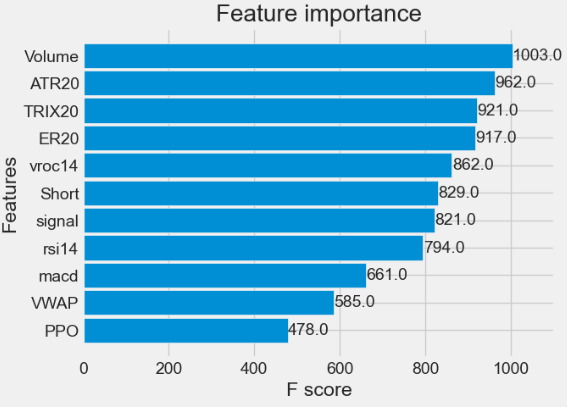
- Printing the key regression metrics
train_mae = mean_absolute_error(y_train, y_train_pred)
test_mae = mean_absolute_error(y_test, y_test_pred)
train_mse = mean_squared_error(y_train, y_train_pred)
test_mse = mean_squared_error(y_test, y_test_pred)
train_r2 = r2_score(y_train, y_train_pred)
test_r2 = r2_score(y_test, y_test_pred)

print(f"Training MAE: {train_mae}")
print(f"Testing MAE: {test_mae}")
print(f"Training MSE: {train_mse}")
print(f"Testing MSE: {test_mse}")
print(f"Training R²: {train_r2}")
print(f"Testing R²: {test_r2}")

Training MAE: 228.24087763538097
Testing MAE: 628.4784233969832
Training MSE: 142584.2164624201
Testing MSE: 1074680.2606905757
Training R²: 0.9993211423118245
Testing R²: 0.9953418575035379- Plotting Actual vs Predicted BTC-USD Close Price for Training and Test Sets as the plt scatter X-plot
plt.figure(figsize=(12, 7))

plt.subplot(1, 2, 1)
plt.scatter(y_train, y_train_pred, alpha=0.3)
plt.xlabel("Actual Close Price (Train)")
plt.ylabel("Predicted Close Price (Train)")
plt.title("Actual vs. Predicted Close Price (Training Set)")
plt.plot([y_train.min(), y_train.max()], [y_train.min(), y_train.max()], "r--")

plt.subplot(1, 2, 2)
plt.scatter(y_test, y_test_pred, alpha=0.3)
plt.xlabel("Actual Close Price (Test)")
plt.ylabel("Predicted Close Price (Test)")
plt.title("Actual vs. Predicted Close Price (Testing Set)")
plt.plot([y_test.min(), y_test.max()], [y_test.min(), y_test.max()], "r--")

plt.tight_layout()
plt.show()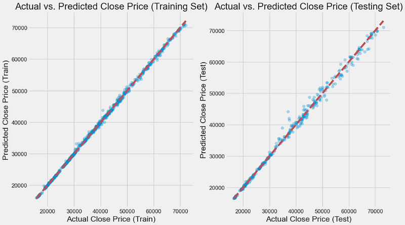
- Comparing predicted vs test BTC-USD Close time series
y_test.plot(label='Test')
plt.scatter(y_test.index,y_test_pred,c='r',label='Predict')
plt.legend()
plt.show()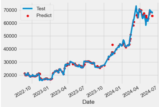
Conclusions
- We have demonstrated how to create a regression pipeline that includes TTI-based feature engineering steps to create new features from existing features by building a reliable ML model using XGBoost.
- This case study has confirmed that Optuna is a powerful and user-friendly Python library for hyperparameter optimization in BTC-USD price prediction with XGBoost regression. Its easy integration, efficient search algorithms, and advanced features make it an invaluable tool for optimizing machine learning models.
- The same considerations apply to other ensemble techniques such as the Random Forest Regression.
- As always, we’ll leave you with some useful references below, so you can expand your pool of knowledge even more and improve your coding skills.
- Stay tuned for more content!
Explore More
- Leveraging Predictive Uncertainties of Time Series Forecasting Models
- A Comprehensive Analysis of Best Trading Technical Indicators w/ TA-Lib — Tesla ‘23
- Multiple-Criteria Technical Analysis of Blue Chips in Python
- Joint Analysis of Bitcoin, Gold and Crude Oil Prices
- BTC-USD Freefall vs FB/Meta Prophet 2022–23 Predictions
- DOGE-INR Price Prediction Backtesting
- BTC-USD Price Prediction with LSTM
- Quant Trading using Monte Carlo Predictions and 62 AI-Assisted Trading Technical Indicators (TTI)
References
- Predictive Analytics in Finance: Utilizing XGBoost for Stock Trend and Price Forecasting
- Predicting Bitcoin price using technical indicator data features in Long short-term Memory models
- XGBoost for stock trend & prices prediction
- Kaggle: XGBoost for stock trend & prices prediction
- Regression | XGBoost + OPTUNA
- Common financial technical indicators implemented in Pandas.
- Algorithmic Trading with ML: BTC Case Study
- Trading with Machine Learning: Classification
- Understanding the Bias-Variance Tradeoff in Machine Learning: Examples and Solutions
- Tutorial: Python for Finance
- Data Science for Financial Markets


