The provided content discusses a comprehensive analysis of 15 different Python algorithms aimed at detecting support and resistance levels (SRL) in the BTC-USD price data, integrating various technical indicators and statistical methods to enhance algo-trading strategies.
Abstract
The text outlines an in-depth exploration of semi-automated detection methods for BTC-USD price support and resistance levels, which are crucial for making informed trading decisions. It details 15 distinct algorithms, ranging from global trend lines and local min/max linear regression to advanced techniques like K-Means clustering and volume-based analysis. The article emphasizes the importance of combining these methods, referred to as the SRL15 approach, to identify not just precise points but also support and resistance zones. This integrative methodology is applied to historical BTC-USD data to demonstrate its potential effectiveness in algorithmic trading, aiming to provide a more systematic approach compared to intuition-based trading.
Opinions
The author, Cristian Velasquez, stresses the significance of integrating multiple methods to reliably identify support and resistance zones rather than exact points.
There is an opinion that the current challenge for BTC-USD is navigating a tight price range, and the Relative Strength Index (RSI) suggests market equilibrium.
The text suggests that market momentum may be slowing down, as indicated by the Market Momentum Slows Amid Trading Hesitation headline.
The author implies that the SRL algorithms could balance the pros and cons of using ambiguous support and resistance zones in crypto trading.
There is a viewpoint that SRL-powered algo-trading might offer a more disciplined approach to BTC trading than one based on instinct or intuition.
The content reflects the idea that the SRL15 methodology could provide a more nuanced understanding of price action by considering both global trends and local price behaviors.
Semi-Automated Detection of BTC-USD Price Support & Resistance Levels: Comparing 15 Essential Methods
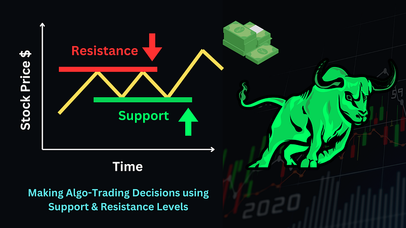
Making Algo-Trading Decisions using Support & Resistance Levels (image design via Canva).
When it comes to stock technical analysis, there is a legion of indicators and SaaS products available. Therefore, it is often useful to combine different tools to get a complete picture of the volatile stock market. Besides, such an integration may offer the proper way to apply the multiple comparison tests.
For example, Fibonacci retracement can be a great tool to use in combination with other technical indicators, as it can provide additional confirmation of support and resistance levels (SRL).
This post is about semi-automated detection of short/long BTC-USD price SRL by combining, evaluating and comparing the following 15 available algorithms in Python [1–15]:
Global Trend Lines
Local MinMax Linear Regression
Candlestick Low/High SRL
Rolling Window Single SRL
Rolling Window Fibonacci Retracement Levels
IQR-Based Multiple SRL
Rolling Window Swing Highs & Lows
Pivot Points with SRL
K-Means Clustering with SRL
Volume-Based SRL
Linear/Polynomial Regression SRL
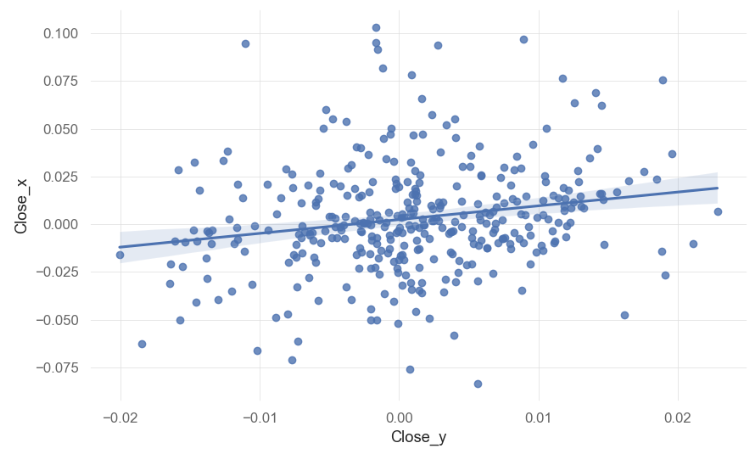
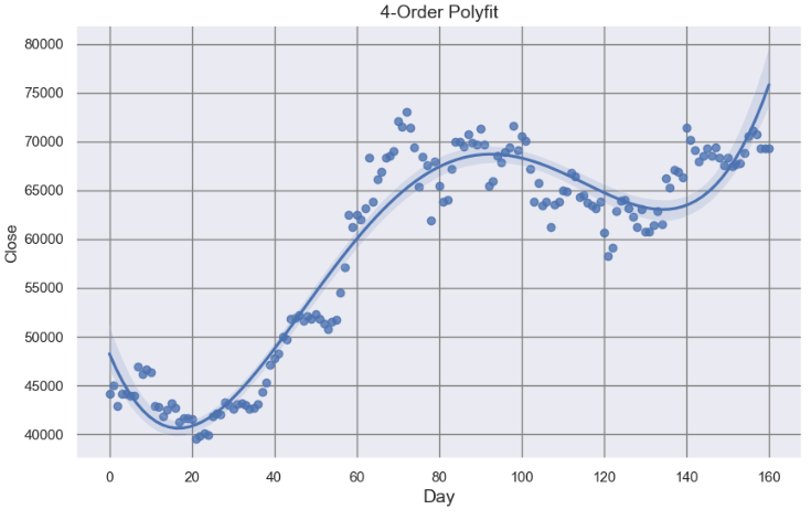
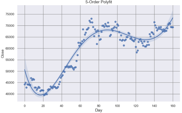
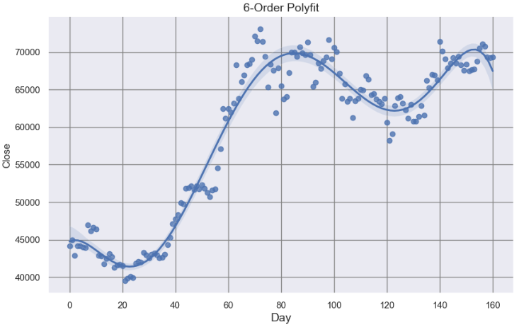
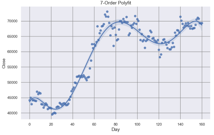
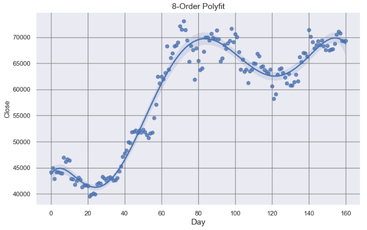
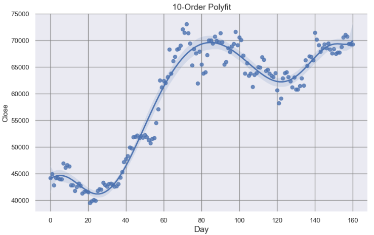
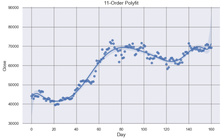
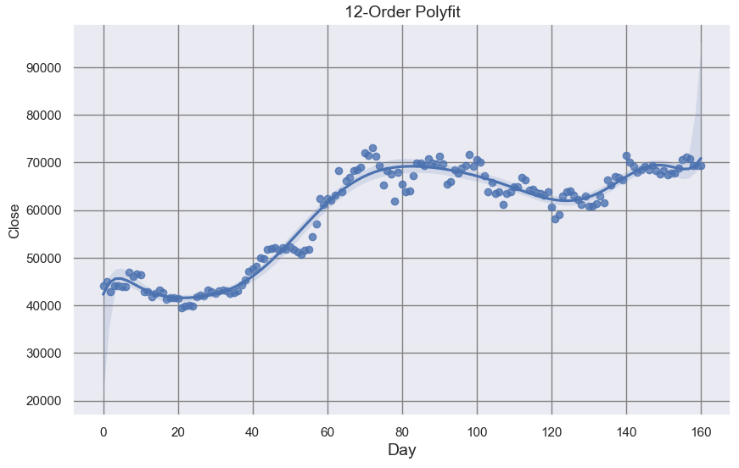
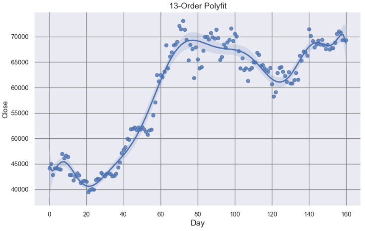
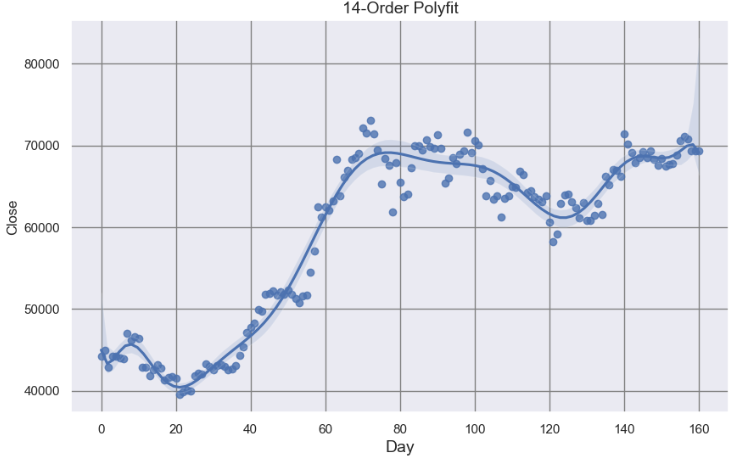
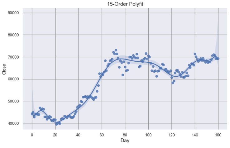
Support-Resistance Visualization QC via Seaborn Polynomial Regression
SMA MinMax Support & Resistance Points
Local Low/High SRL
Global Low/High SRL
As Cristian Velasquez points out in his article [1], the importance of integration of the aforementioned methods to reliably identify support and resistance zones rather than precise points cannot be overstated.
For BTC-USD, the current challenge is the tight price range that it has been navigating in for some time now. On the daily chart, BTC has been oscillating between the $60k and $70k marks, struggling to find a definitive direction. The Relative Strength Index (RSI), situated around the 50% level, implies equilibrium in market momentum.
Can the SRL-powered algo-trading provide a more systematic approach to BTC trading than one based on intuition or instinct?
Can the SRL algorithms [1–15] help us to balance pros & cons of using ambiguoussupport and resistance zones in crypto trading?
Let’s try to address these questions by diving into the specifics of the proposed integrated methodology (being referred to as SRL15) to be demonstrated on BTC-USD historical data.
Support & Resistance Basics
SRL in crypto trading aretwo elementary concepts concerning technical analysis. At the core, these are the price levels that act as barriers to price movement.
Identifying SRL involves recognizing price thresholds in the market where an asset often stops or changes direction due to a significant amount of buying or selling.
Support Level: This is a price below an asset that usually does not fall. When the price approaches this zone, traders expect the asset to become attractive enough to buy.
Resistance Level: This is a price zone above which the price usually does not rise. Reaching this zone is often seen by traders as a sell signal, expecting the price to fall due to the rise in supply.
Consider bouncing a ball around your house. Your floor and ceiling are barriers limiting the ball’s flight and fall. Support and resistance are similar barriers in trading that limit the movement of price action.
The crypto trading strategy based on support and resistance levels is the following: buy slightly above the support in the uptrends and sell near the resistance in downtrends.
Remember, there’s no assurance that the support and resistance will hold, take an extra step and wait until the trends confirmation. Combine support and resistance levels with other indicators that confirm the trend.
Read more about support and resistance with examples and strategies here.
Reading & Plotting Input Stock Data
Importing and installing basic Python libraries
import os
os.chdir('YOURPATH')    # Set working directory
os. getcwd()

import warnings
warnings.filterwarnings('ignore')

import numpy as np
import pandas as pd
from datetime import datetime as dt
import yfinance as yf
import nsepy
from statistics import mean
Reading the short-term BTC-USD historical stock data
benchmark_ = ["BTC-USD"]
start_date_ = "2024-01-01"
end_date_ = "2024-06-10"
df = yf.download(benchmark_, start=start_date_, end=end_date_)
df.tail()
Open High Low Close Adj Close Volume
Date
2024-06-05 70568.35156271735.41406270390.71093871082.82031271082.820312328107714092024-06-06 71082.84375071625.73437570119.12500070757.16406270757.164062252231520072024-06-07 70759.18750071907.85156268507.25781269342.58593869342.585938361883810962024-06-08 69324.17968869533.32031269210.74218869305.77343869305.773438142621858612024-06-09 69297.49218869408.93750069160.84375069312.34375069312.34375012721441792
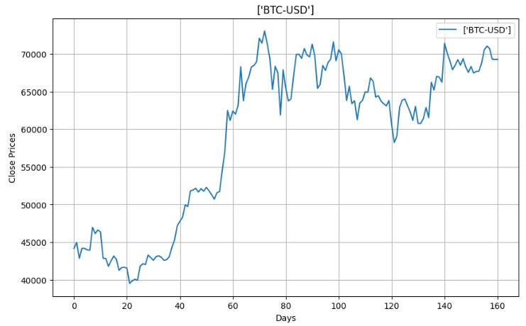
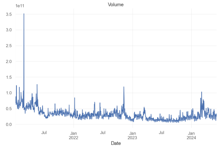
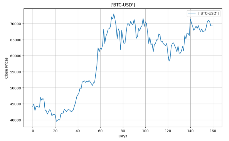
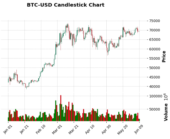
Plotting the short-term BTC-USD historical stock data
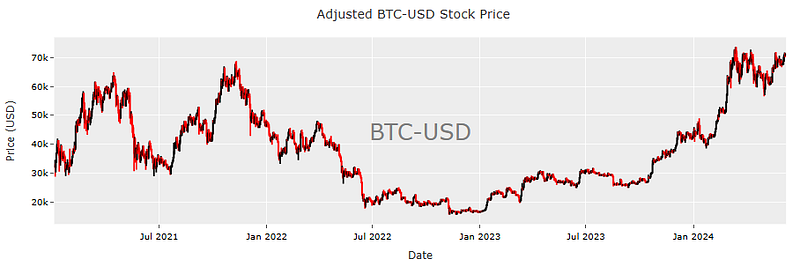
The long-term BTC-USD historical stock data candlestick chart
Common Risk/Return FinTech Analysis
Importing stock data analysis libraries
# Importing Libraries# Data Handlingimport pandas as pd
import numpy as np
# Data Visualizationimport matplotlib.pyplot as plt
import seaborn as sns
import plotly.express as px
import plotly.graph_objs as go
import matplotlib.ticker as mtick
from plotly.offline import init_notebook_mode
init_notebook_mode(connected=True)
# Financial Data Analysisimport yfinance as yf
import ta
import quantstats as qs
# Machine Learning from sklearn.metrics import roc_auc_score, roc_curve, auc
# Modelsfrom sklearn.linear_model import LogisticRegression
from xgboost import XGBClassifier
from lightgbm import LGBMClassifier
from catboost import CatBoostClassifier
from sklearn.ensemble import AdaBoostClassifier, RandomForestClassifier
# Hiding warnings import warnings
warnings.filterwarnings("ignore")
Reading the long-term BTC-USD data
benchmark_ = ["BTC-USD"]
start_date_ = "2021-01-03"
end_date_ = "2024-06-08"
df = yf.download(benchmark_, start=start_date_, end=end_date_)
df.tail()
Open High Low Close Adj Close Volume
Date
2024-06-03 67753.89843870230.82031267589.83593868804.78125068804.781250324012853242024-06-04 68804.57031271047.40625068564.64062570567.76562570567.765625331496965452024-06-05 70568.35156271735.41406270390.71093871082.82031271082.820312328107714092024-06-06 71082.84375071625.73437570119.12500070757.16406270757.164062252231520072024-06-07 70772.41406271432.11718870672.61718871216.85937571216.85937526067939328
Printing the basic descriptive statistics of Adj Close price
# Get the number of days
days = (df.index[-1] - df.index[0]).days
# Calculate the CAGR
cagr = ((((df['Adj Close'][-1]) / df['Adj Close'][1])) ** (365.0/days)) - 1# Print CAGRprint(cagr)
0.25343289151250503
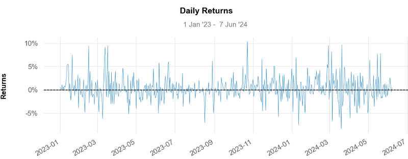
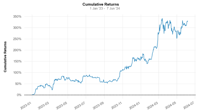
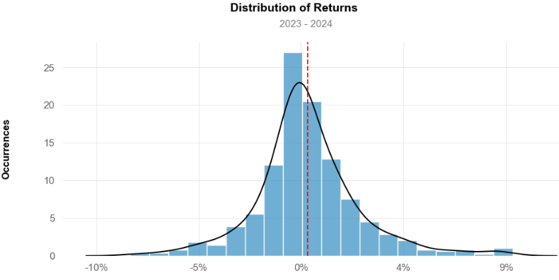
Calculating daily and cumulative returns for the time slot 2023–2024
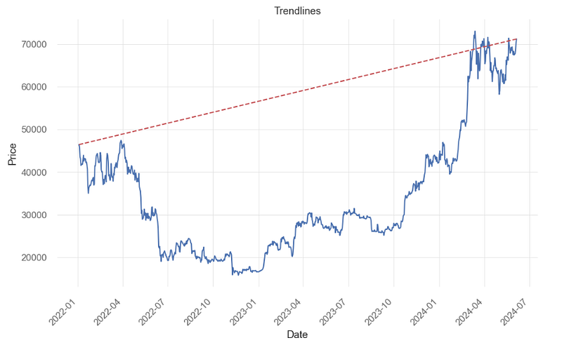
Let’s select the time slot from start=’2022–01–01' to end=’2024–06–09' and draw trend lines connecting significant highs or lows to visualize the simplest global trend direction
import yfinance as yf
import matplotlib.pyplot as plt
data = yf.download('BTC-USD', start='2022-01-01', end='2024-06-09')
# Dropping values with missing/null values
data = data.dropna()

# Drawing a simple trendline
plt.plot(data['Close'])
plt.plot([data.index[0], data.index[-1]], [data['Close'].iloc[0], data['Close'].iloc[-1]], 'r--')

# Rotate x-axis dates
plt.xticks(rotation=45, ha='right')

# Add labels and title
plt.xlabel('Date')
plt.ylabel('Price')
plt.title('Trendlines')
BTC-USD Simplest Global Trendlines
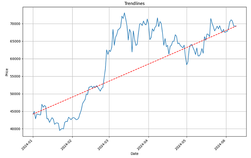
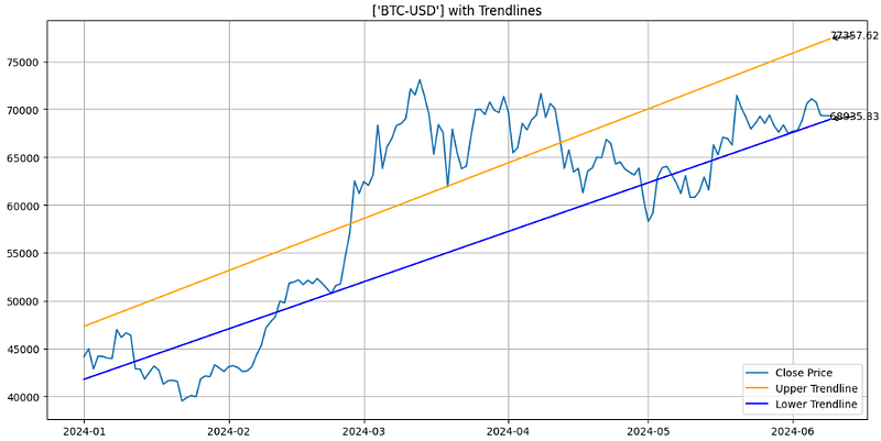
Selecting the shorter time slot 2024/01–06 and re-estimating the aforementioned trendlines
import warnings
warnings.filterwarnings('ignore')

import numpy as np
import pandas as pd
from datetime import datetime as dt
import yfinance as yf
import nsepy
from statistics import mean

benchmark_ = ["BTC-USD"]

start_date_ = "2024-01-01"
end_date_  = "2024-06-10"

df = yf.download(benchmark_, start=start_date_, end=end_date_)
#df.tail()

data = df.copy()


# Drawing a simple trendline
plt.figure(figsize=(12, 7))
plt.plot(data['Close'])
plt.plot([data.index[0], data.index[-1]], [data['Close'].iloc[0], data['Close'].iloc[-1]], 'r--')

# Rotate x-axis dates
plt.xticks(rotation=45, ha='right')

# Add labels and title
plt.xlabel('Date')
plt.ylabel('Price')
plt.title('Trendlines')
plt.grid()
BTC-USD Simplest Global Trendlines 2024
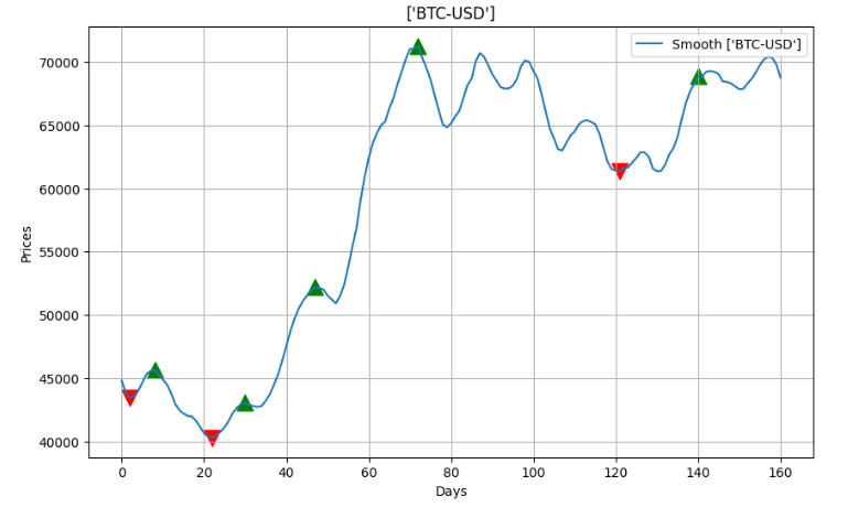
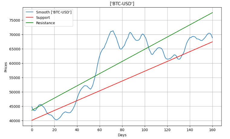
Method 2: Local MinMax Linear Regression
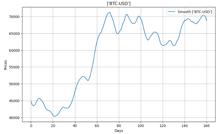
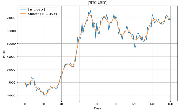
Applying linear regression and local MinMax search to the smoothed BTC-USD data 2024 (see above)
import numpy as np
import pandas as pd
from math import sqrt
import matplotlib.pyplot as plt
import pandas_datareader as web
from scipy.signal import savgol_filter
from sklearn.linear_model import LinearRegression
defpythag(pt1, pt2):
a_sq = (pt2[0] - pt1[0]) ** 2
b_sq = (pt2[1] - pt1[1]) ** 2return sqrt(a_sq + b_sq)
defregression_ceof(pts):
X = np.array([pt[0] for pt in pts]).reshape(-1, 1)
y = np.array([pt[1] for pt in pts])
model = LinearRegression()
model.fit(X, y)
return model.coef_[0], model.intercept_
deflocal_min_max(pts):
local_min = []
local_max = []
prev_pts = [(0, pts[0]), (1, pts[1])]
for i inrange(1, len(pts) - 1):
append_to = ''if pts[i-1] > pts[i] < pts[i+1]:
append_to = 'min'elif pts[i-1] < pts[i] > pts[i+1]:
append_to = 'max'if append_to:
if local_min or local_max:
prev_distance = pythag(prev_pts[0], prev_pts[1]) * 0.5
curr_distance = pythag(prev_pts[1], (i, pts[i]))
if curr_distance >= prev_distance:
prev_pts[0] = prev_pts[1]
prev_pts[1] = (i, pts[i])
if append_to == 'min':
local_min.append((i, pts[i]))
else:
local_max.append((i, pts[i]))
else:
prev_pts[0] = prev_pts[1]
prev_pts[1] = (i, pts[i])
if append_to == 'min':
local_min.append((i, pts[i]))
else:
local_max.append((i, pts[i]))
return local_min, local_max
defisSupport(df,i):
support = df['Low'][i] < df['Low'][i-1] and df['Low'][i] < df['Low'][i+1] \
and df['Low'][i+1] < df['Low'][i+2] and df['Low'][i-1] < df['Low'][i-2]
return support
defisResistance(df,i):
resistance = df['High'][i] > df['High'][i-1] and df['High'][i] > df['High'][i+1] \
and df['High'][i+1] > df['High'][i+2] and df['High'][i-1] > df['High'][i-2]
return resistance
levels = []
for i inrange(2,df.shape[0]-2):
if isSupport(df,i):
levels.append((i,df['Low'][i]))
elif isResistance(df,i):
levels.append((i,df['High'][i]))
defplot_all():
fig, ax = plt.subplots()
candlestick_ohlc(ax,df.values,width=0.6, \
colorup='green', colordown='red', alpha=0.8)
date_format = mpl_dates.DateFormatter('%d %b %Y')
ax.xaxis.set_major_formatter(date_format)
fig.autofmt_xdate()
fig.tight_layout()
for level in levels:
plt.hlines(level[1],xmin=df['Date'][level[0]],\
xmax=max(df['Date']),colors='blue')
fig.show()
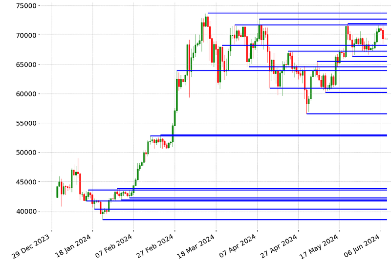
plot_all()
BTC-USD Candlestick Chart 2024/01–06 with Local Low/High SRL
Method 4: Rolling Window Single Support & Resistance Lines
Invoking the Rolling Midpoint Range SRL algorithm [1]
import numpy as np
import pandas as pd
import yfinance as yf
import matplotlib.pyplot as plt
deffind_levels(data, window):
high = data['High'].rolling(window=window).max()
low = data['Low'].rolling(window=window).min()
midpoint = (high + low) / 2
diff = high - low
resistance = midpoint + (diff / 2)
support = midpoint - (diff / 2)
return support, resistance
# Download historical stock prices 2024/01–06 (see above)
data = df.copy()
window = 30# Calculate support and resistance levels
support, resistance = find_levels(data, window)
# Plot the stock price, support, and resistance lines
fig, ax = plt.subplots(figsize=(12, 6))
ax.plot(data.index, data['Close'], label='Stock Price')
ax.plot(data.index, support, label='Support', linestyle='--', color='green')
ax.plot(data.index, resistance, label='Resistance', linestyle='--', color='red')
ax.set_xlabel('Date')
ax.set_ylabel('Price')
ax.set_title(f'{symbol} Stock Price with Support and Resistance Levels')
ax.legend()
# Add annotations for last support and resistance levels
last_support = support.iloc[-1]
last_resistance = resistance.iloc[-1]
ax.annotate(f'Support: {last_support:.2f}', xy=(support.index[-1], last_support),
xytext=(support.index[-1] - pd.DateOffset(days=30), last_support + 10),
arrowprops=dict(facecolor='green', arrowstyle='->'))
ax.annotate(f'Resistance: {last_resistance:.2f}', xy=(resistance.index[-1], last_resistance),
xytext=(resistance.index[-1] - pd.DateOffset(days=30), last_resistance - 10),
arrowprops=dict(facecolor='red', arrowstyle='->'))
plt.grid()
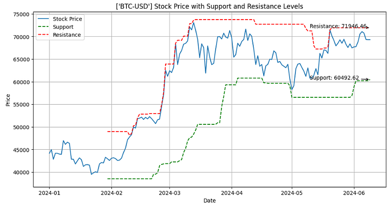
plt.show()
BTC-USD Price 2024/01–06: the Rolling Midpoint Range SRL
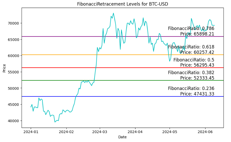
Method 5: Rolling Window Fibonacci Retracement Levels
The Fibonacci retracement levels are 23.6%, 38.2%, 61.8%, and 78.6%. While not officially a Fibonacci ratio, 50% is also used. The indicator is useful because it can be drawn between any two significant price points, such as a high and a low.
We will notice that when we plot Fibonacci retracement levels on our charts they align beautifully with significant highs and lows. These high-probability areas act as perfect entry or exit points for trades because they have proven over time to show where price has reversed from a new trend.
Method 5.1 (Local): Calculating the high and low prices over the lookback period of 15 [1]
stock_data = df.copy()
# Define the lookback period for calculating high and low prices
lookback_period = 15# Calculate the high and low prices over the lookback period
high_prices = stock_data["High"].rolling(window=lookback_period).max()
low_prices = stock_data["Low"].rolling(window=lookback_period).min()
Fibonacci Retracement Levels for BTC-USD 2024/01–06 using the global Max/Min of Adj Close
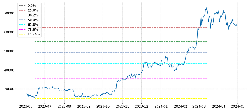
Method 5.3 (Global): Consider the long-term BTC-USD historical stock dataset (see above) to define the Highest/Lowest Swings and the adjusted time period within these Swings [1]
highest_swing = -1
lowest_swing = -1for i inrange(1,df.shape[0]-1):
if df['High'][i] > df['High'][i-1] and df['High'][i] > df['High'][i+1] and (highest_swing == -1or df['High'][i] > df['High'][highest_swing]):
highest_swing = i
if df['Low'][i] < df['Low'][i-1] and df['Low'][i] < df['Low'][i+1] and (lowest_swing == -1or df['Low'][i] < df['Low'][lowest_swing]):
lowest_swing = i
ratios = [0,0.236, 0.382, 0.5 , 0.618, 0.786,1]
colors = ["black","r","g","b","cyan","magenta","yellow"]
levels = []
max_level = df['High'][highest_swing]
min_level = df['Low'][lowest_swing]
for ratio in ratios:
if highest_swing > lowest_swing: # Uptrend
levels.append(max_level - (max_level-min_level)*ratio)
else: # Downtrend
levels.append(min_level + (max_level-min_level)*ratio)
plt.rcParams['figure.figsize'] = [18, 8]
plt.rc('font', size=14)
plt.plot(df['Close'])
start_date = df.index[min(highest_swing,lowest_swing)]
end_date = df.index[max(highest_swing,lowest_swing)]
for i inrange(len(levels)):
plt.hlines(levels[i],start_date, end_date,label="{:.1f}%".format(ratios[i]*100),colors=colors[i], linestyles="dashed")
plt.legend()
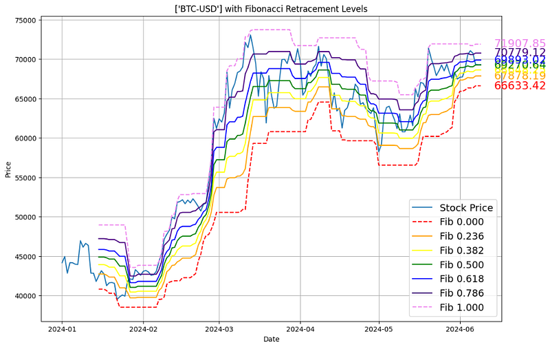
plt.show()
Fibonacci Retracement Levels for BTC-USD using the Highest/Lowest Swings and the adjusted time frame
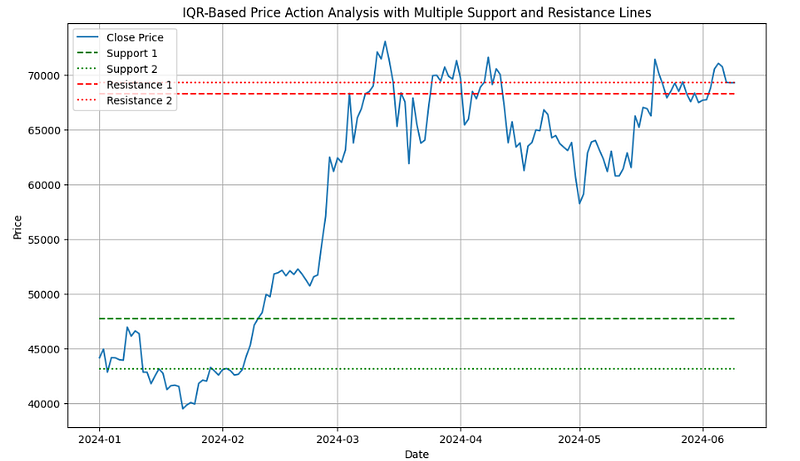
Method 6: IQR-Based Global Multiple Support & Resistance Lines
The interquartile range (IQR) is the difference between the third quartile and first quartile of a stock price.
Using IQR as a statistical measure that helps to determine the spread of prices in quartiles.
Assuming we have our data 2024/01–06 in a DataFrame named ‘data’
data=df.copy()
Defining 2 main SRL via 25th and 75th percentiles
# Example: using 25th and 75th percentiles
support = data['Close'].quantile(0.25)
resistance = data['Close'].quantile(0.75)
Defining 2 additional SRL via 15th and 85th percentiles
# Plotting
plt.figure(figsize=(12, 7))
# Plotting Close Price
plt.plot(data['Close'], label='Close Price')
# Plotting Support Lines
plt.hlines(support, xmin=data.index[0], xmax=data.index[-1], colors='green', linestyles='dashed', label='Support 1')
plt.hlines(support_2, xmin=data.index[0], xmax=data.index[-1], colors='green', linestyles='dotted', label='Support 2')
# Add more support lines as needed using adjusted variable names# Plotting Resistance Lines
plt.hlines(resistance, xmin=data.index[0], xmax=data.index[-1], colors='red', linestyles='dashed', label='Resistance 1')
plt.hlines(resistance_2, xmin=data.index[0], xmax=data.index[-1], colors='red', linestyles='dotted', label='Resistance 2')
# Add more resistance lines as needed using adjusted variable names# Displaying Legends
plt.legend()
# Add labels and title
plt.title('IQR-Based Price Action Analysis with Multiple Support and Resistance Lines')
plt.xlabel('Date')
plt.ylabel('Price')
plt.grid()
plt.show()
BTC-USD Price 2024/01–06: IQR-Based Price Action Analysis with Multiple Support and Resistance Lines
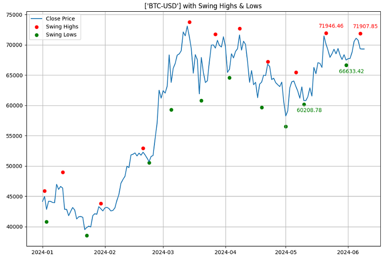
Method 7: Rolling Window Swing Highs & Lows
Swing highs and swing lows are earlier market turning points. Hence, they are natural choices for projecting support and resistance levels. Every swing point is a potential support or resistance level.
Detecting and plotting local Min/Max (Swings) [1]
#Swing Highs and Lowsimport yfinance as yf
import pandas as pd
from scipy.signal import argrelextrema
import matplotlib.pyplot as plt
# Download stock data
stock_data = df.copy()
# Identify local maxima (swing highs)
stock_data['Swing_High'] = stock_data['High'][argrelextrema(stock_data['High'].values, np.greater_equal, order=5)[0]]
# Identify local minima (swing lows)
stock_data['Swing_Low'] = stock_data['Low'][argrelextrema(stock_data['Low'].values, np.less_equal, order=5)[0]]
# Find last two non-NaN values for Swing Highs and Swing Lows
last_two_resistances = stock_data['Swing_High'].dropna().tail(2)
last_two_supports = stock_data['Swing_Low'].dropna().tail(2)
# Plotting
plt.figure(figsize=(12,8))
plt.plot(stock_data['Close'], label="Close Price")
plt.scatter(stock_data.index, stock_data['Swing_High'], color='r', label='Swing Highs', marker='o')
plt.scatter(stock_data.index, stock_data['Swing_Low'], color='g', label='Swing Lows', marker='o')
# Annotate the last two resistance and support pricesfor date, price in last_two_resistances.items():
plt.annotate(f"{price:.2f}", (date, price), textcoords="offset points", xytext=(10,10), ha='center', color='r')
for date, price in last_two_supports.items():
plt.annotate(f"{price:.2f}", (date, price), textcoords="offset points", xytext=(10,-15), ha='center', color='g')
plt.title(f'{symbol} with Swing Highs & Lows')
plt.legend()
plt.grid()
plt.show()
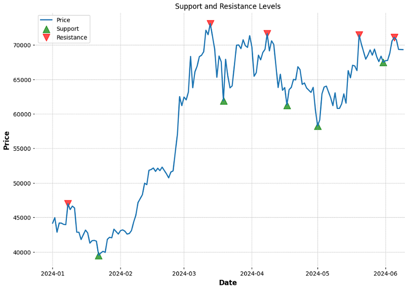
BTC-USD Price 2024/01–06 with Swing Highs & Lows
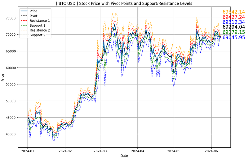
Method 8: Pivot Points with Support & Resistance Lines
Pivot points SRL are widely accepted as the simplest yet most effective trading strategy. The pivot point is the point in which the market sentiment changes from bearish to bullish.
BTC-USD Price 2024/01–06 with Pivot Points and SRL
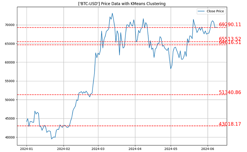
Method 9: K-Means Clustering with Support & Resistance Lines
Using the K-Means clustering algorithm to detect SRL (cf. [5]).
The K-means clustering algorithm finds different sections of the time series data, and groups them into a defined number of groups. This number (K) can be optimized. The highest and lowest value of each group is then defined as the support and resistance values for the cluster.
Method 9.1: Global K-Means Price Clustering [1] is implemented as follows:
#K-Means Price Clusteringimport yfinance as yf
import numpy as np
import matplotlib.pyplot as plt
from sklearn.cluster import KMeans
# Download BTC-USD stock data 2024
stock_data = df.copy()
# Preparing data for clustering: Normalize time and price to have similar scales
X_time = np.linspace(0, 1, len(stock_data)).reshape(-1, 1)
X_price = (stock_data['Close'].values - np.min(stock_data['Close'])) / (np.max(stock_data['Close']) - np.min(stock_data['Close']))
X_cluster = np.column_stack((X_time, X_price))
# Applying KMeans clustering
num_clusters = 5
kmeans = KMeans(n_clusters=num_clusters)
kmeans.fit(X_cluster)
# Extract cluster centers and rescale back to original price range
cluster_centers = kmeans.cluster_centers_[:, 1] * (np.max(stock_data['Close']) - np.min(stock_data['Close'])) + np.min(stock_data['Close'])
# Plotting
plt.figure(figsize=(12,8))
plt.plot(stock_data['Close'], label="Close Price")
for center in cluster_centers:
plt.axhline(y=center, color='r', linestyle='--')
plt.annotate(f"{center:.2f}", xy=(stock_data.index[-1], center * 1.01), xytext=(5,0), textcoords="offset points", fontsize=15, ha='left', va='center', color='r')
plt.title(f'{symbol} Price Data with KMeans Clustering')
plt.legend()
plt.grid()
plt.show()
BTC-USD Price 2024: Global K-Means Clustering SRL
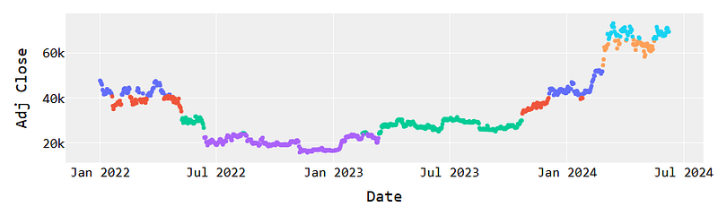
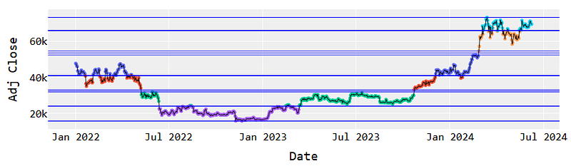
Method 9.2: Calculating SRL using Local K-Means Clustering
# Long-term BTC-USD data 2022-2024 (see above)
btc = df.copy()
# Convert adjusted closing price to numpy array
btc_prices = np.array(btc["Adj Close"])
print("BTC Prices:\n", btc_prices)
# Perform cluster analysis
K = 6
kmeans = KMeans(n_clusters=6).fit(btc_prices.reshape(-1, 1))
# predict which cluster each price is in
clusters = kmeans.predict(btc_prices.reshape(-1, 1))
#print("Clusters:\n", clusters)# Assigns plotly as visualization engineimport plotly.graph_objects as go
pd.options.plotting.backend = 'plotly'# Arbitrarily 6 colors for our 6 clusters
colors = ['red', 'orange', 'yellow', 'green', 'blue', 'indigo']
# Create Scatter plot, assigning each point a color based# on it's grouping where group_number == index of color.
fig = btc.plot.scatter(
x=btc.index,
y="Adj Close",
color=[colors[i] for i in clusters],
)
# Configure some styles
layout = go.Layout(
plot_bgcolor='#efefef',
showlegend=False,
# Font Families
font_family='Monospace',
font_color='#000000',
font_size=20,
xaxis=dict(
rangeslider=dict(
visible=False
))
)
fig.update_layout(layout)
# Display plot in local browser window
fig.show()
K-Means Clustering of Long-term BTC-USD 2022–2024
Calculating Local MinMax price values within K-Means clusters
# Create list to hold values, initialized with infinite values
min_max_values = []
# init for each cluster groupfor i inrange(6):
# Add values for which no price could be greater or less
min_max_values.append([np.inf, -np.inf])
# Print initial valuesprint(min_max_values)
# Get min/max for each clusterfor i inrange(len(btc_prices)):
# Get cluster assigned to price
cluster = clusters[i]
# Compare for min valueif btc_prices[i] < min_max_values[cluster][0]:
min_max_values[cluster][0] = btc_prices[i]
# Compare for max valueif btc_prices[i] > min_max_values[cluster][1]:
min_max_values[cluster][1] = btc_prices[i]
# Print resulting valuesprint(min_max_values)
[[inf, -inf], [inf, -inf], [inf, -inf], [inf, -inf], [inf, -inf], [inf, -inf]]
[[65980.8125, 73083.5], [33086.234375, 40826.21484375], [15787.2841796875, 23957.529296875], [40951.37890625, 52284.875], [24136.97265625, 31792.310546875], [54522.40234375, 65738.7265625]]
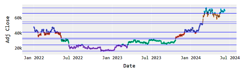
Plotting horizontal SRL associated with the above clusters
import plotly.graph_objects as go
# Again, assign an arbitrary color to each of the 6 clusters
colors = ['red', 'orange', 'yellow', 'green', 'blue', 'indigo']
# Create Scatter plot, assigning each point a color where# point group = color index.
fig = btc.plot.scatter(
x=btc.index,
y="Adj Close",
color=[colors[i] for i in clusters],
)
# Add horizontal linesfor cluster_min, cluster_max in min_max_values:
fig.add_hline(y=cluster_min, line_width=1, line_color="blue")
fig.add_hline(y=cluster_max, line_width=1, line_color="blue")
# Add a trace of the price for better clarity
fig.add_trace(go.Trace(
x=btc.index,
y=btc['Adj Close'],
line_color="black",
line_width=1
))
# Make it pretty
layout = go.Layout(
plot_bgcolor='#efefef',
showlegend=False,
# Font Families
font_family='Monospace',
font_color='#000000',
font_size=20,
xaxis=dict(
rangeslider=dict(
visible=False
))
)
fig.update_layout(layout)
fig.show()
Horizontal SRL associated with the K-Means clusters
Appending more MinMax values within the K-Means clusters
print("Initial Min/Max Values:\n", min_max_values)
# Create container for combined values
output = []
# Sort based on cluster minimum
s = sorted(min_max_values, key=lambda x: x[0])
# For each cluster get average offor i, (_min, _max) inenumerate(s):
# Append min from first clusterif i == 0:
output.append(_min)
# Append max from last clusterif i == len(min_max_values) - 1:
output.append(_max)
# Append average from cluster and adjacent for all otherselse:
output.append(sum([_max, s[i+1][0]]) / 2)
print("Sorted Min/Max Values:\n", output)
Initial Min/Max Values:
[[65980.8125, 73083.5], [33086.234375, 40826.21484375], [15787.2841796875, 23957.529296875], [40951.37890625, 52284.875], [24136.97265625, 31792.310546875], [54522.40234375, 65738.7265625]]
Sorted Min/Max Values:
[15787.2841796875, 24047.2509765625, 32439.2724609375, 40888.796875, 53403.638671875, 65859.76953125, 73083.5]
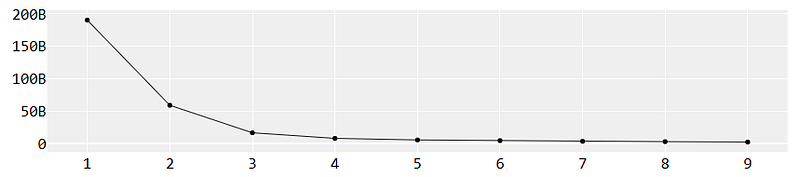
Checking K-means clusters with K=10
# create a list to contain output values
values = []
# Define a range of cluster values to assess
K = range(1, 10)
# Performa a clustering using each value, save inertia_ value from eachfor k in K:
kmeans_n = KMeans(n_clusters=k)
kmeans_n.fit(btc_prices.reshape(-1, 1))
values.append(kmeans_n.inertia_)
Examining the Elbow Plot
import plotly.graph_objects as go
# Create initial figure
fig = go.Figure()
# Add line plot of inertia values
fig.add_trace(go.Trace(
    x=list(K),
    y=values,
    line_color="black",
    line_width=1
))
# Make it pretty
layout = go.Layout(
    plot_bgcolor='#efefef',
    showlegend=False,
    # Font Families
    font_family='Monospace',
    font_color='#000000',
    font_size=20,
    xaxis=dict(
        rangeslider=dict(
            visible=False
        ))
)
fig.update_layout(layout)
fig.show()
BTC-USD K-Means Elbow Plot
Plotting updated horizontal SRL vs K-Means clusters of BTC-USD Adj Close 2022–2024
import plotly.graph_objects as go
# Again, assign an arbitrary color to each of the 6 clusters
colors = ['red', 'orange', 'yellow', 'green', 'blue', 'indigo']
# Create Scatter plot, assigning each point a color where# point group = color index.
fig = btc.plot.scatter(
x=btc.index,
y="Adj Close",
color=[colors[i] for i in clusters],
)
# Add horizontal linesfor cluster_min, cluster_max in min_max_values:
fig.add_hline(y=cluster_min, line_width=1, line_color="blue")
fig.add_hline(y=cluster_max, line_width=1, line_color="blue")
# Add a trace of the price for better clarity
fig.add_trace(go.Trace(
x=btc.index,
y=btc['Adj Close'],
line_color="black",
line_width=1
))
# Make it pretty
layout = go.Layout(
plot_bgcolor='#efefef',
showlegend=False,
# Font Families
font_family='Monospace',
font_color='#000000',
font_size=20,
xaxis=dict(
rangeslider=dict(
visible=False
))
)
# Add horizontal linesfor cluster_avg in output:
fig.add_hline(y=cluster_avg, line_width=1, line_color="blue")
fig.update_layout(layout)
fig.show()
Horizontal Local SRL vs K-Means clusters of BTC-USD Adj Close 2022–2024
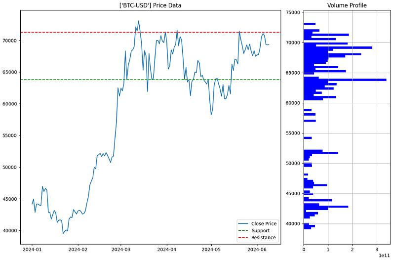
Method 10: Volume-Based Support & Resistance Lines
Remember the importance of trading volume, which can confirm the strength of each level, as changes in volume often signal the reliability of support or resistance.
The algorithm [1] consists of the following steps: (1) calculate the volume profile in terms of the 100 price bins Low/High Min/Max; (2) calculate SRL based on np.digitize(current_price, price_bins); (3) plotting price with SRL vs Volume profile, viz.
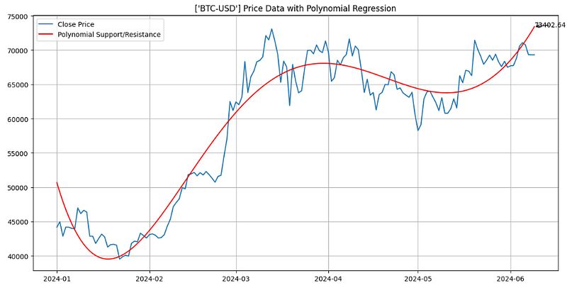
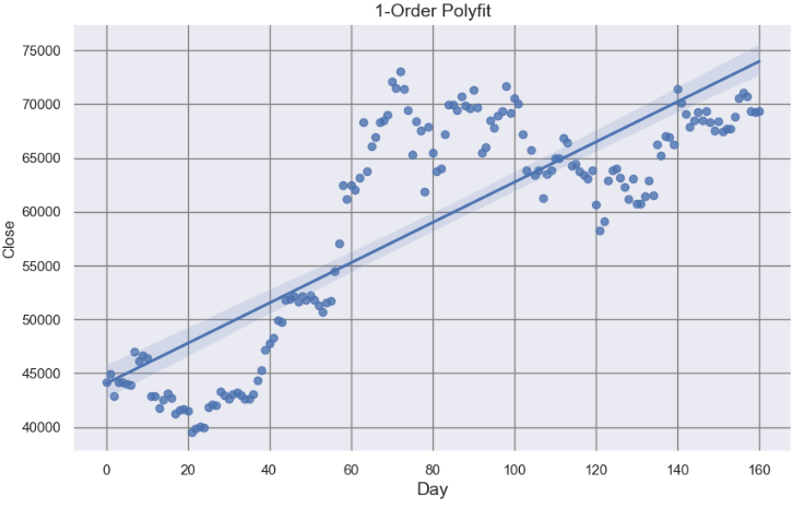
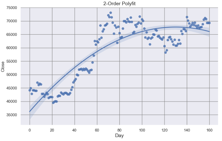
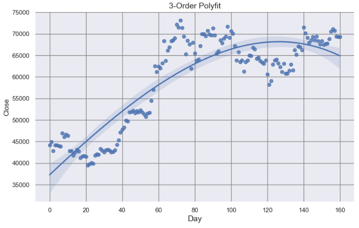
Method 11: Linear/Polynomial Regression Support & Resistance Lines
A linear regression channel consists of a median line with 2 parallel lines, above and below it, at the same distance. Those lines can be seen as support and resistance.
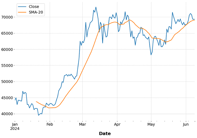
Moving averages are a popular technical indicator that can be used in combination with Fibonacci retracement. Moving averages can help identify the trend of the market, while Fibonacci retracement can provide key support and resistance levels.
For example, if the price is above the 200-day moving average, and the retracement level is at the 50% level, traders can confirm that the trend is bullish and enter a buy position.
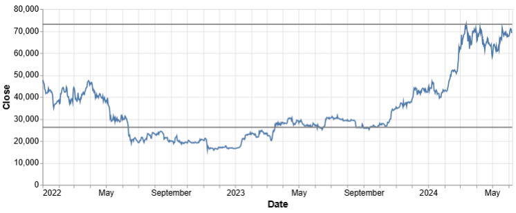
But what is the optimal (or statistically significant) SMA window length? Here is the answer:
These 2 levels are denoted by multiple touches of price without a breakthrough of the level in 2024.
Conclusions
In this comprehensive case study, we have explored various types of SRL. This includes pivot-based, Fibonacci, global/local MinMax, trend lines, rolling window, low/high, swing highs & lows, SMA, IQR, K-Means clustering, horizontal, and diagonal single/multiple levels.
Specifically, we have utilized the BTC-USD historical data to evaluate 15 essential SRL methods within the context of automated algo-trading technical analysis discussed earlier [1–15].
The resulting integrated SRL15 approach represents our guiding light in the world of crypto trading. It helps us manage the BTC’s volatility and risks effectively.
For quant traders: placing stops and limits below support and above resistance zones detected by SRL15 is strongly recommended.
Another strategy used in SRL trading is the breakout strategy, whereby traders wait for the stock price to move outside either level.
Pros: Traders can aim to sell a particular asset when the price reaches a resistance level zone. This indicates a potential reversal of the uptrend and a good opportunity to sell at a higher price.
Cons: SRL are generally unreliable indicators of future price movements. SRL zones can be broken if there is a significant shift in market sentiment or other factors that influence crypto markets.
Our results have shown that support and resistance are crucial risk management concepts necessary to make informed decisions in crypto trading and maximize profits.
Using these essential technical analysis tools, cryptocurrency traders can identify potential entry and exit points.
Disclaimer: Although SRL can provide crucial insights into price movements, traders should incorporate other technical analysis tools and fundamental analysis to develop a well-rounded trading strategy. These methods can reduce the risk of missed opportunities or false signals.
The following disclaimer clarifies that the information provided in this article is for educational use only and should not be considered financial or investment advice.
The information provided does not take into account your individual financial situation, objectives, or risk tolerance.
Any investment decisions or actions you undertake are solely your responsibility.
You should independently evaluate the suitability of any investment based on your financial objectives, risk tolerance, and investment timeframe.
It is recommended to seek advice from a certified financial professional who can provide personalized guidance tailored to your specific needs.
The tools, data, content, and information offered are impersonal and not customized to meet the investment needs of any individual. As such, the tools, data, content, and information are provided solely for informational and educational purposes only.