
LSTM Model For Apple Stock Prediction
In this technical exploration, we apply a Long Short-Term Memory (LSTM) model to predict Apple Inc.’s stock prices, leveraging Python’s robust data science ecosystem. Key steps involve importing libraries like Numpy, Pandas, and hvplot for data handling and visualization, followed by data preprocessing which includes reading, cleaning, and feature extraction from Apple’s stock data (AAPL.csv) with Twitter sentiment scores. We then employ window-based feature engineering, split the data for training and testing, and standardize it using MinMaxScaler. The LSTM model, built using Keras, undergoes training and evaluation using metrics such as Root Mean Squared Error and R-squared. The process culminates in a visual comparison of predicted versus actual stock values, showcasing LSTM’s efficacy in financial time series prediction.
#Importing Libraries
import numpy as np
import pandas as pd
import hvplot.pandas
%matplotlib inline
from sklearn import metrics
The Python code snippet is a preparatory step in setting up an environment for algorithmic trading analysis. It begins by importing various libraries and functionalities that are pivotal for data manipulation, analysis, and visualization. First, numpy imported as np is a fundamental package for numerical computing in Python. Its widely used in algorithmic trading for handling large multidimensional arrays and matrices, alongside a collection of mathematical functions to operate on these arrays. Next, pandas imported as pd is a library providing high-performance, easy-to-use data structures and data analysis tools. In the context of algorithmic trading, it is often used for handling and analyzing financial time series data. The hvplot.pandas import suggests the use of the hvplot library, a high-level plotting API built on HoloViews that provides an alternative to the built-in pandas plotting functionality. This allows creating interactive plots ideally suited for analyzing financial data in a dynamic and insightful manner. The %matplotlib inline command is a magic function for the IPython environment that enables the inline display of plots created by matplotlib, a popular plotting library. This means graphs will be shown directly beneath the code cells within a Jupyter Notebook, an ideal feature for quick visual analysis during trading algorithm development. Lastly, from sklearn import metrics shows that the code will utilize the metrics module from the scikit-learn library abbreviated as sklearn. This module provides functions for calculating performance metrics of the algorithmic models, essential for evaluating their predictions regarding trading strategies.
# Set the random seed for reproducibility
from numpy.random import seed

seed(1)
from tensorflow import random

random.set_seed(2)
This Python code snippet serves to set fixed seed values for the random number generators used in NumPy and TensorFlow. This is often done to ensure that the results of running the code are reproducible; that is, every time the code is run, it will produce the same results. This is particularly important in algorithmic trading where the consistency of strategy evaluation or model training is crucial for assessing its performance and making decisions based on those assessments. In algorithmic trading, strategies often rely on random processes for aspects such as portfolio allocation, order execution timing, or sampling of market data. By fixing the random seeds at the beginning of the code, any randomness in these processes will follow the same sequence for each run, which allows the developer to isolate the effects of code changes from the randomness in the simulations or models.
# Read APPL.csv contains open, high, low, close, Adj close, Volume of Apple stock with twitter polarity scores and twitter volume
df = pd.read_csv('AAPL.csv', index_col="Date", infer_datetime_format=True, parse_dates=True)

# Drop null values
df.dropna(inplace=True)
df.tail()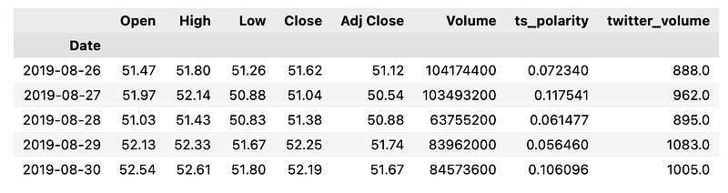
The code reads a CSV file named AAPL.csv, which contains historical trading data for Apple Inc. referred to by its ticker symbol, AAPL. The CSV file includes several columns: open, high, low, close, adjusted close prices, trading volume, twitter polarity scores, and twitter volume. The polarity scores and twitter volume suggest an element of sentiment analysis based on Twitter data, likely to assess public sentiment towards Apples stock. The pd.read_csv function from the Pandas library is used to read the file, with the Date column set as the index of the resulting DataFrame, which implies that each row of data corresponds to a specific date. The infer_datetime_format=True argument helps Pandas to automatically detect and interpret the format of the date strings in the Date column, while parse_dates=True instructs the reader to convert the date strings into Python datetime objects, which are suitable for time-series analysis. After reading the data into a DataFrame, the code then drops any rows with missing values by calling df.dropna. This cleaning step is essential to ensure the quality of the data, especially since algorithmic trading models require accurate inputs to make reliable trading decisions. Lastly, df.tail is used to display the last few rows of the DataFrame, which is often done to verify that the data has been loaded correctly and to provide a quick glimpse of the most recent data points.
# Dataframe with Adj close, ts_polarity, twitter_volume of APPL
df = df[["Adj Close", "ts_polarity", "twitter_volume"]]
df.head()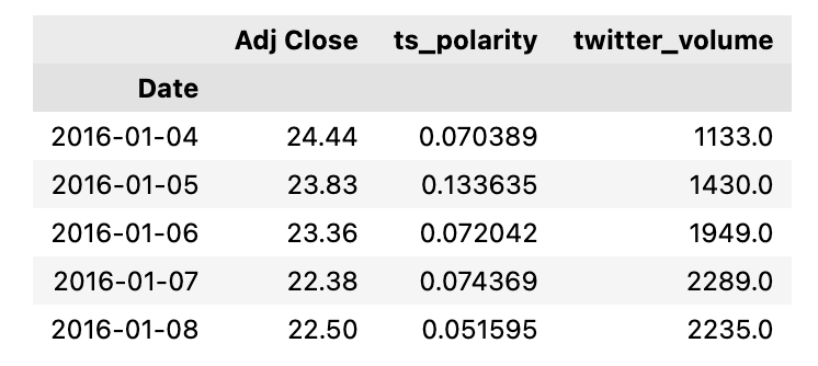
The code is manipulating a dataframe, likely obtained from a data analysis or manipulation library such as pandas. The dataframe df is being modified to only include three columns: Adj Close, ts_polarity, and twitter_volume, which pertain to the stock of Apple Inc. APPL. Adj Close likely represents the adjusted closing price of Apples stock, which accounts for any corporate actions like dividends and stock splits. ts_polarity could represent a sentiment analysis score derived from Twitter data, indicating whether the sentiment of tweets about Apple is positive, negative, or neutral. twitter_volume likely captures the volume of tweets about Apple, indicating the level of Twitter activity or buzz around the company. Finally, the snippet calls the .head method on the dataframe, which would display the first few usually five rows of the modified dataframe. This is generally used to quickly inspect the top rows of the dataset to ensure it looks correct after the modification. The overall purpose of this code segment is to prepare and inspect a subset of data that might be used to make trading decisions based on the stock price, sentiment analysis from Twitter, and the volume of Twitter discussions surrounding Apples stock. These data points could feed into algorithmic trading models that aim to predict stock price movements and execute trades automatically based on such analyses.
# pct change based on Adj close value
df["Pct_change"] = df["Adj Close"].pct_change()

# Drop null values
df.dropna(inplace = True)
df.head()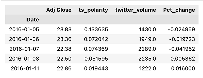
The adjusted closing price takes into account factors such as dividends, stock splits, and other corporate actions, providing a more accurate reflection of a securitys value over time. The first line of the code creates a new column in a DataFrame named df called Pct_change. This new column is populated with the percentage change of the adjusted close prices between each row and the previous row. The pct_change function is a Pandas method applied to the Adj Close column that automatically calculates this change. The second line of code removes any rows in the DataFrame that contain null or missing values, which could result from the pct_change function the first row will be NA since there is no previous row to compare to. This cleanup is necessary because null values can interfere with trading algorithms and analyses by introducing inaccuracies. The final part, df.head, is a method that, if this were part of a script with additional context, would display the first few rows of the cleaned and updated DataFrame. This is useful for verifying the data processing steps or for quick inspection of the transformed data.
Creating The Features X and Target y Data
The initial step in data preparation involved creating the input features, labeled as X, and the target vector, referred to as y. This was done using the window data function. This function is designed to break down the data using a rolling window method. It uses a rolling window defined by Xt minus window to predict the value of Xt.
The window data function produces two types of numpy arrays. The first is X, which contains the input feature vectors. The second is y, which is the target vector. These arrays are essential for the later stages of data analysis and prediction modeling.
The function comes with several parameters for customization. The first parameter is df, which stands for the original DataFrame that contains the time series data. This data is crucial for the creation of the feature and target vector. The window parameter defines the window size in days and determines the range of previous closing prices used for prediction. The feature col number parameter indicates the column number in the original DataFrame where the features are found. Finally, the target col number parameter points out the column in the DataFrame where the target data is located. This helps the function accurately extract the required data for the target vector.
# This function "window_data" accepts the column number for the features (X) and the target (y)
# It chunks the data up with a rolling window of Xt-n to predict Xt
# It returns a numpy array of X any y
def window_data(df, window, feature_col_number1, feature_col_number2, feature_col_number3, target_col_number):
    # Create empty lists "X_close", "X_polarity", "X_volume" and y
    X_close = []
    X_polarity = []
    X_volume = []
    y = []
    for i in range(len(df) - window):

        # Get close, ts_polarity, tw_vol, and target in the loop
        close = df.iloc[i:(i + window), feature_col_number1]
        ts_polarity = df.iloc[i:(i + window), feature_col_number2]
        tw_vol = df.iloc[i:(i + window), feature_col_number3]
        target = df.iloc[(i + window), target_col_number]

        # Append values in the lists
        X_close.append(close)
        X_polarity.append(ts_polarity)
        X_volume.append(tw_vol)
        y.append(target)

    return np.hstack((X_close,X_polarity,X_volume)), np.array(y).reshape(-1, 1)
This Python code defines a function called window_data that prepares data for use in algorithmic trading. The purpose of the code is to organize historical trading data into a format that can be used to train a machine learning model to predict future price movements. It involves creating input features X and a target variable y to be used in model training. The function takes as inputs a DataFrame df, a window size window, and column numbers which represent different types of market data such as the closing price, sentiment polarity, and trading volume. It creates rolling windows of historical data points for each of these features, along with the future value of the target variable that needs to be predicted. The function iterates over the DataFrame, collecting slices of data for each feature column within the specified window size. These slices correspond to sequential periods in the financial time series dataset. For each iteration, it appends the collected slices to their respective lists: closing prices to X_close, sentiment polarity to X_polarity, and trading volume to X_volume. Simultaneously, it also collets the target variable, which is the value to predict at the end of each window period, appending it to the list y. Finally, the function combines the lists of input features into a single two-dimensional NumPy array where each feature is a column, and it reshapes the list of target variables to create a two-dimensional NumPy array as well. Both arrays are then returned by the function for use in further analysis or model training.
# Predict Closing Prices using a 3 day window of previous closing prices
window_size = 3

# Column index 0 is the `Adj Close` column
# Column index 1 is the `ts_polarity` column
# Column index 2 is the `twitter_volume` column
feature_col_number1 = 0
feature_col_number2 = 1
feature_col_number3 = 2
target_col_number = 0
X, y = window_data(df, window_size, feature_col_number1, feature_col_number2, feature_col_number3, target_col_number)
The code utilizes a function called window_data to create datasets based on a specified window size of three days. The window_data function is applied to a dataframe df that presumably contains historical stock data. Using a moving window of three days, the function extracts features and the target variable from the dataframe. The features include the adjusted closing price Adj Close, a sentiment polarity score based on related tweets ts_polarity, and the volume of tweets mentioning the stock twitter_volume. These features are selected based on their column indexes in the dataframe. The target variable for prediction is also the adjusted closing price of the stock. The outcome of this function is to generate a set of input features X and the corresponding target y to be used for training a predictive model. This model could then be used to forecast future closing prices of the stock, informing trading decisions.
# Use 70% of the data for training and the remaineder for testing
X_split = int(0.7 * len(X))
y_split = int(0.7 * len(y))

X_train = X[: X_split]
X_test = X[X_split:]
y_train = y[: y_split]
y_test = y[y_split:]
The data appears to be divided into features X and target values y. The code first determines the split point for both the features and target datasets, aiming to use 70% of the data for training. It calculates an index that corresponds to 70% of the length of X and y, respectively. Using these indices, it splits X and y into two parts each: one part for training 70% of the data and one part for testing the remaining 30% of the data. After executing this code, you would have four subsets: X_train and y_train which are used to train the algorithm, and X_test and y_test which are used to test or validate the performance of the trading model. The training set helps the model learn the patterns, while the testing set is necessary to evaluate how well the model performs on data it hasnt seen before. This practice aims to prevent overfitting and ensures the models robustness and generalization ability.
Scaling Data With MinMaxScaler
# Use the MinMaxScaler to scale data between 0 and 1.
x_train_scaler = MinMaxScaler()
x_test_scaler = MinMaxScaler()
y_train_scaler = MinMaxScaler()
y_test_scaler = MinMaxScaler()

# Fit the scaler for the Training Data
x_train_scaler.fit(X_train)
y_train_scaler.fit(y_train)

# Scale the training data
X_train = x_train_scaler.transform(X_train)
y_train = y_train_scaler.transform(y_train)

# Fit the scaler for the Testing Data
x_test_scaler.fit(X_test)
y_test_scaler.fit(y_test)

# Scale the y_test data
X_test = x_test_scaler.transform(X_test)
y_test = y_test_scaler.transform(y_test)
The purpose of this code is to scale the input features X and the target values y into a range between 0 and 1, which is often done to standardize the range of independent variables for optimal performance in machine learning models. The code creates instances of the MinMaxScaler, a tool from the scikit-learn library, for both the training and testing data. It then fits the scalers to the respective datasets, meaning it calculates the minimum and maximum values of the data which will be used for scaling. After fitting, the training and testing data points are transformed by the scaler, effectively scaling them within the specified range 0 to 1 in this case. This is done so that all features contribute equally to the distance computation in algorithms that are sensitive to the scale of the data, like gradient descent-based and distance-based algorithms. It is particularly important in trading algorithms where the magnitude of the data can vary widely.
Reshape Features Data For The LSTM Model
# Reshape the features for the model
X_train = X_train.reshape((X_train.shape[0], X_train.shape[1], 1))
X_test = X_test.reshape((X_test.shape[0], X_test.shape[1], 1))
Specifically, its adjusting the shape of the training and testing datasets, also known as feature sets, to make them compatible with the requirements of a certain type of model that expects input data to have a specific number of dimensions. The code uses the .reshape method to transform the datasets X_train for training and X_test for testing. It is converting the data into a 3D format, with the new shape being the size of the dataset along the first dimension the number of samples, the original feature dimension the number of input variables or time steps, depending on context along the second dimension, and adding a third dimension with a size of 1. In algorithmic trading, such reshaping is commonly performed when preparing data for models like Convolutional Neural Networks CNNs or Long Short-Term Memory networks LSTMs that expect input data to have multiple dimensions. By reshaping the data, the code is ensuring that the input features are in the correct form to be fed into the model for training or prediction. This is crucial for the model to learn patterns from the data and make informed trading decisions based on those patterns.
Build And Train The LSTM RNN
# Build the LSTM model.

# Define the LSTM RNN model.
model = Sequential()

number_units = 9
dropout_fraction = 0.2

# Layer 1
model.add(LSTM(
    units=number_units,
    return_sequences=True,
    input_shape=(X_train.shape[1], 1))
    )

model.add(Dropout(dropout_fraction))

# Layer 2
# The return_sequences parameter needs to set to True every time we add a new LSTM layer, excluding the final layer.
model.add(LSTM(units=number_units, return_sequences=True))
model.add(Dropout(dropout_fraction))

# Layer 3
model.add(LSTM(units=number_units))
model.add(Dropout(dropout_fraction))

# Output layer
model.add(Dense(1))
The Python code snippet outlines the structure for an LSTM Long Short-Term Memory RNN Recurrent Neural Network model. LSTM models are a specialized kind of RNN that are well-suited to making predictions based on time series data, which makes them useful for algorithmic trading where past stock prices or financial indicators can be used to forecast future prices. This particular model is being built with the Keras deep learning library as is indicated by the use of Sequential for initializing the model and the subsequent stacking of layers with add. The LSTM layers are designed to allow the network to learn dependencies at different time scales, with dropout introduced after each LSTM layer to prevent overfitting. Dropout randomly sets a fraction of the input units to 0 at each update during training, which helps in making the model generalization better. The model consists of three LSTM layers, where the first two layers return sequences; this indicates that their full output is retained and used as input for the subsequent layer. The third LSTM layer does not return sequences, implying its output is provided only at the end, which is typically done before the final layer in a sequence prediction model. The final dense layer has a single neuron which output the predicted value for the time series.
Compiling The LSTM RNN Model
# Compile the model
model.compile(optimizer="adam", loss="mean_squared_error")
The model, after being defined with a particular architecture, is being compiled with specified optimizer and loss function parameters. The optimizer adam is a popular algorithm used in training neural networks, and it is responsible for adjusting the weights of the network through the learning process to minimize the predictive error. Adam stands for Adaptive Moment Estimation and combines the advantages of two other extensions of stochastic gradient descent, namely Adaptive Gradient Algorithm AdaGrad and Root Mean Square Propagation RMSProp. The loss function mean_squared_error is a common choice for regression problems and measures the average of the squares of the errors — that is, the average squared difference between the estimated values and the actual value. In the context of algorithmic trading, this would typically measure how far the models predictions of financial metrics, such as price, are from the true values. The purpose of the loss function is to guide the optimizer by providing a quantitative measure of the models performance. Overall, the purpose of this code is to prepare the neural network for the training phase, where it will learn to predict certain outcomes from data, which in the case of algorithmic trading would include predicting stock prices, market movements, or other financial indicators that could inform trading decisions. Once the model is compiled, it can then be trained with historical data and subsequently used to make informed trades.
# Summarize the model
model.summary()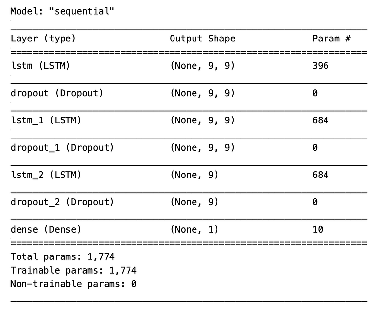
The model.summary function call is used to provide a quick overview of the models layers, their shapes, and the number of parameters they each have both trainable and non-trainable. This is useful for verifying the architecture of a neural network or a similar predictive model used in the context of trading strategies. The purpose of the code is to present an at-a-glance understanding of the complexity and design of the model, which can be pertinent when adjusting the model or diagnosing issues with its performance. By knowing the summarized details of the model, developers and data scientists can ensure that the model meets the expectations for the given trading algorithm and is appropriate for the data it will analyze. This is an important step in refining and validating the machine learning aspect of algorithmic trading systems.
Training The Model
# Train the model
model.fit(X_train, y_train, epochs=10, shuffle=False, batch_size=5, verbose=1)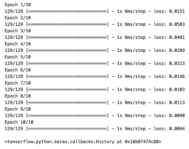
The purpose of this code is to fit the model to a set of training data so that it can learn patterns from historical trading information, which it might then use to make predictions or decisions about future trades. The model.fit function is used to train the model on the provided input features X_train and the target values y_train. The training process will iterate through the dataset in a number of runs specified by epochs. In this case, epochs=10 means the model will go through the training dataset ten times. The training data will not be shuffled between epochs, which is indicated by shuffle=False. Shuffling data is often done to ensure that the model does not learn anything from the order of the data. batch_size=5 specifies that the model should update its parameters learn after every five samples. Finally, verbose=1 means that the training process will output a detailed log to the console, including information about the progress of the training, the loss, and any other metrics the model might be tracking. By fine-tuning the model through this training process, the aim is to create an efficient algorithm for trading that can provide decisions to buy or sell financial instruments, such as stocks, based on predictions that stem from historical price and possibly other financial data.
Model Performance
# Make some predictions
predicted = model.predict(X_test)
The method predict is called on the model object, passing X_test as an argument. X_test likely contains feature data formatted in a way that the model can interpret. These features could be technical indicators, historical prices, or other market data relevant to algorithmic trading. The purpose of this code is to generate output from the model based on input data X_test, where the output is referred to as predicted. The predicted variable presumably stores the models predictions regarding future stock prices, price movements, or other financial metrics relevant to trading decisions. In the context of algorithmic trading, the predictions made by the model could be used to inform trading strategies. For instance, the model might predict future price increases or decreases of stocks, and these predictions could lead to automated decisions to buy, sell, or hold certain securities in a trading portfolio. The effectiveness of the model in making accurate predictions would be critical to the success of such trading strategies.
# Evaluating the model
print('Root Mean Squared Error:', np.sqrt(metrics.mean_squared_error(y_test, predicted)))
print('R-squared :', metrics.r2_score(y_test, predicted))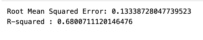
The model has been trained to forecast future prices or movements in the financial market and it has made predictions for a set of test data. The code calculates two important evaluation metrics: Root Mean Squared Error RMSE and R-squared R². RMSE is a measure of the average magnitude of the errors between the predicted values from the model and the actual values observed in the test data, while R² is a statistical measure of how well the regression predictions approximate the real data points. By printing these two metrics, the code is essentially providing a quantitative assessment of the models accuracy: RMSE gives an indication of the error magnitude, with lower values indicating better fit, and R² represents the proportion of the variance in the dependent variable that is predictable from the independent variables, with values closer to 1 indicating a better predictive performance.
# Create a DataFrame of Real and Predicted values
stocks = pd.DataFrame({
    "Real": real_prices.ravel(),
    "Predicted": predicted_prices.ravel()
}, index = df.index[-len(real_prices): ])
stocks.head()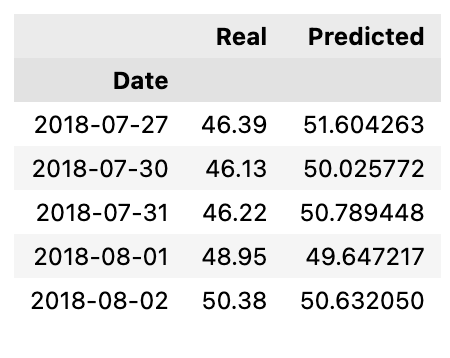
The code creates a new DataFrame called stocks with two columns: Real and Predicted. The Real column is filled with actual stock prices that have been flattened into a one-dimensional array using the ravel method. Similarly, the Predicted column contains predicted stock prices, also flattened. The index for the new DataFrame is set to match the dates or timestamps of the original data from which the real prices were extracted. Specifically, it uses the same index as the last entries of the original data df that correspond in number to the length of the real_prices array, ensuring that each row in the stocks DataFrame has an associated date or time. Finally, the stocks.head function call displays the first few rows of the DataFrame, providing a quick look at the top entries to verify the structure and data. The purpose of this code is to facilitate a comparative analysis of real and predicted stock price data, likely for an algorithmic trading strategy. By organizing this information into a neat tabular format, it makes it easier to visualize, analyze, and backtest the performance of the predictive model against actual market data.
# Plot the real vs predicted values as a line chart
stocks.hvplot(title = "Real vs Predicted values of APPL")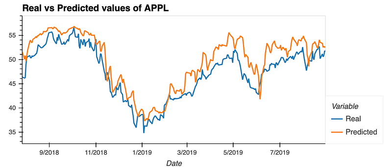
It uses the hvplot library, which is a high-level plotting API built on the HoloViews library that provides an alternative to Matplotlib and Seaborn for creating interactive plots. With the .hvplot function, a line chart is generated with a title Real vs Predicted values of APPL. This visualization helps in assessing the accuracy of a predictive model in algorithmic trading by comparing the models predictions against known stock prices. The line chart could make it straightforward for a user to spot discrepancies between the real and predicted values over time, enabling the user to evaluate and possibly improve the predictive model.


