Day 13 of 30 days of Data Engineering Series with Projects

Welcome back peeps to Day 13 of Data Engineering Series with Projects!

In this we will cover —

Pandas

Data Cleaning and processing

Outlier Detection

Noisy Data

Missing Data

Pandas Functions

Aggregate Functions

Joins

Pre-requisite to Day 12 is to complete Day 1–11( link below):

Day 1 : What’s Data Engineering, Why Data Engineering, Data Engineers — ML Engineers — Data Scientists, Purpose and Scope

Day 2 : Complete Python for Data Engineering — Part 1

Day 3 : Complete Advanced Python for Data Engineering — Part 2

Day 4: Techniques to write efficient and Optimized Code

Day 5 : SQL

Day 6 : Advanced SQL

Day 7 : BigQuery and SQL vs NOSQL databases

Day 8 : Advanced Functions

Day 9 : Query Optimizations

Day 10 : MySQL and PostgreSQL

Day 11: Shell scripting and Linux “touch” command

Day 12 : Map Reduce, Data Warehouse, Data Lakes

Day 13: Pandas, Pandas, Data Cleaning and processing, Outlier Detection, Noisy Data, Missing Data, Pandas Functions, Aggregate Functions, Joins

Projects Videos —

All the projects, data structures, SQL, algorithms, system design, Data Science and ML , Data Analytics, Data Engineering, , Implemented Data Science and ML projects, Implemented Data Engineering Projects, Implemented Deep Learning Projects, Implemented Machine Learning Ops Projects, Implemented Time Series Analysis and Forecasting Projects, Implemented Applied Machine Learning Projects, Implemented Tensorflow and Keras Projects, Implemented PyTorch Projects, Implemented Scikit Learn Projects, Implemented Big Data Projects, Implemented Cloud Machine Learning Projects, Implemented Neural Networks Projects, Implemented OpenCV Projects,Complete ML Research Papers Summarized, Implemented Data Analytics projects, Implemented Data Visualization Projects, Implemented Data Mining Projects, Implemented Natural Leaning Processing Projects, MLOps and Deep Learning, Applied Machine Learning with Projects Series, PyTorch with Projects Series, Tensorflow and Keras with Projects Series, Scikit Learn Series with Projects, Time Series Analysis and Forecasting with Projects Series, ML System Design Case Studies Series videos will be published on our youtube channel ( just launched).

Subscribe today!

Tech Newsletter —

If you are interested, you can join my newsletter through which I send tech interview tips, techniques, patterns, hacks — Software Development, ML, Data Science, Startups and Technology projects to more than 30K readers. You can subscribe to Ignito:

System Design Case Studies — In Depth

Design Instagram

Design Netflix

Design Reddit

Design Amazon

Design Messenger App

Design Twitter

Design URL Shortener

Design Dropbox

Design Youtube

Design API Rate Limiter

Design Web Crawler

Design Amazon Prime Video

Design Facebook’s Newsfeed

Design Yelp

Design Uber

Design Tinder

Design Tiktok

Design Whatsapp

Most Popular System Design Questions

Mega Compilation : Solved System Design Case studies

This is Day 13 of 30 days of Data Engineering Series where we will be covering —

Pandas

Let’s get started!

Pandas is a powerful library in Python for data manipulation and analysis. It provides a wide range of functions for data cleaning and processing, including:

• Data Cleaning:Dropping unnecessary columns or rows
• Replacing missing or incorrect values with more appropriate ones
• Formatting and normalizing data
• Handling duplicate data
• Outlier Detection:Using the “describe()” function to identify extreme values
• Using visualization techniques like box plots or scatter plots to detect outliers
• Using statistical methods like Z-scores or the Interquartile Range (IQR) to identify outliers
• Noisy Data:Removing or replacing incorrect or irrelevant data
• Using techniques like data smoothing or data normalization to reduce noise
• Missing Data:Identifying missing data with functions like “isnull()” or “notnull()”
• Filling in missing data with values like the mean, median, or mode
• Using interpolation or extrapolation methods to fill in missing data

Pandas also provides a wide range of aggregate functions for data analysis, such as:

• Sum, Mean, Median, Mode
• Min, Max
• Count, Count unique
• Standard deviation, Variance

Joins are used to combine data from multiple tables. Pandas provide different types of joins like:

• Inner Join
• Left Join
• Right Join
• Outer Join

These functions can be used on dataframes to combine the data based on the matching keys.

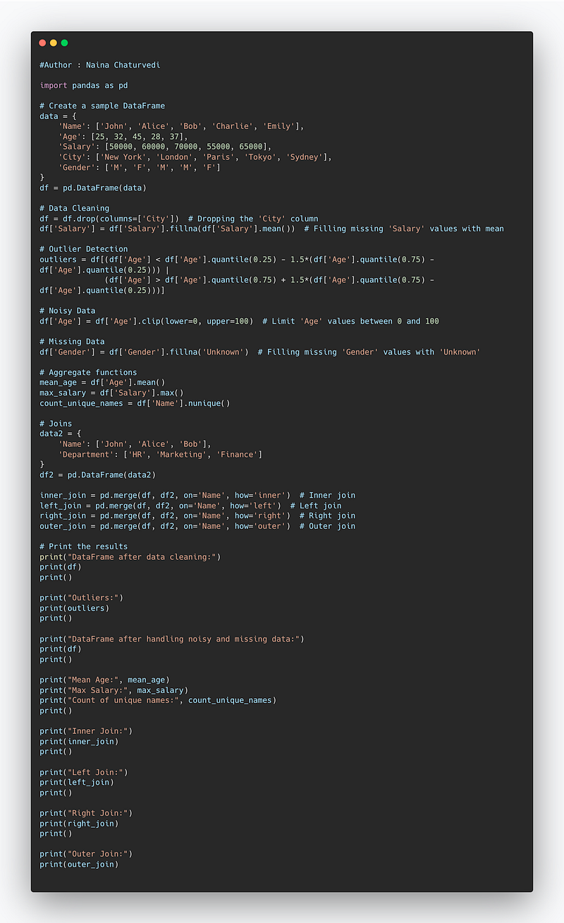
Code Implementation —

import pandas as pd

# Create a sample DataFrame
data = {
    'Name': ['John', 'Alice', 'Bob', 'Charlie', 'Emily'],
    'Age': [25, 32, 45, 28, 37],
    'Salary': [50000, 60000, 70000, 55000, 65000],
    'City': ['New York', 'London', 'Paris', 'Tokyo', 'Sydney'],
    'Gender': ['M', 'F', 'M', 'M', 'F']
}
df = pd.DataFrame(data)

# Data Cleaning
df = df.drop(columns=['City'])  # Dropping the 'City' column
df['Salary'] = df['Salary'].fillna(df['Salary'].mean())  # Filling missing 'Salary' values with mean

# Outlier Detection
outliers = df[(df['Age'] < df['Age'].quantile(0.25) - 1.5*(df['Age'].quantile(0.75) - df['Age'].quantile(0.25))) |
              (df['Age'] > df['Age'].quantile(0.75) + 1.5*(df['Age'].quantile(0.75) - df['Age'].quantile(0.25)))]

# Noisy Data
df['Age'] = df['Age'].clip(lower=0, upper=100)  # Limit 'Age' values between 0 and 100

# Missing Data
df['Gender'] = df['Gender'].fillna('Unknown')  # Filling missing 'Gender' values with 'Unknown'

# Aggregate functions
mean_age = df['Age'].mean()
max_salary = df['Salary'].max()
count_unique_names = df['Name'].nunique()

# Joins
data2 = {
    'Name': ['John', 'Alice', 'Bob'],
    'Department': ['HR', 'Marketing', 'Finance']
}
df2 = pd.DataFrame(data2)

inner_join = pd.merge(df, df2, on='Name', how='inner')  # Inner join
left_join = pd.merge(df, df2, on='Name', how='left')  # Left join
right_join = pd.merge(df, df2, on='Name', how='right')  # Right join
outer_join = pd.merge(df, df2, on='Name', how='outer')  # Outer join

# Print the results
print("DataFrame after data cleaning:")
print(df)
print()

print("Outliers:")
print(outliers)
print()

print("DataFrame after handling noisy and missing data:")
print(df)
print()

print("Mean Age:", mean_age)
print("Max Salary:", max_salary)
print("Count of unique names:", count_unique_names)
print()

print("Inner Join:")
print(inner_join)
print()

print("Left Join:")
print(left_join)
print()

print("Right Join:")
print(right_join)
print()

print("Outer Join:")
print(outer_join)

Snippet —

Let’s deep dive !

Pandas is a a fast, powerful, flexible and easy to use open source data analysis and manipulation tool. It’s a newer package built on top of NumPy, and provides an efficient implementation of a DataFrame.

DataFrames are essentially multidimensional arrays with attached row and column labels, and often with heterogeneous types and/or missing data.

Pandas —

It’s an open source Python package written for the Python programming language for data manipulation, analysis and ML tasks

It is built on top of another package named Numpy, which provides support for mathematical computations and multi-dimensional arrays.

For Data Science and ML projects —

Some of the other best Series —

30 Days of Natural Language Processing ( NLP) Series

30 days of Data Structures and Algorithms and System Design Simplified

60 Days of Deep Learning with Projects Series

60 days of Data Science and ML Series with projects

Data Science and Machine Learning Research ( papers) Simplified **

100 days : Your Data Science and Machine Learning Degree Series with projects

23 Data Science Techniques You Should Know

Tech Interview Series — Curated List of coding questions

Complete System Design with most popular Questions Series

Complete Data Visualization and Pre-processing Series with projects

Kaggle Best Notebooks that will teach you the most

Complete Developers Guide to Git

All the Data Science and Machine Learning Resources

210 Machine Learning Projects

30 days of Machine Learning Ops

Tech Newsletter —

If you are interested, you can join my newsletter through which I send tech interview tips, techniques, patterns, hacks — Software Development, ML, Data Science, Startups and Technology projects to more than 30K readers. You can subscribe to Tech Brew :

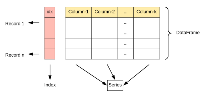
Pandas Series and DataFrame

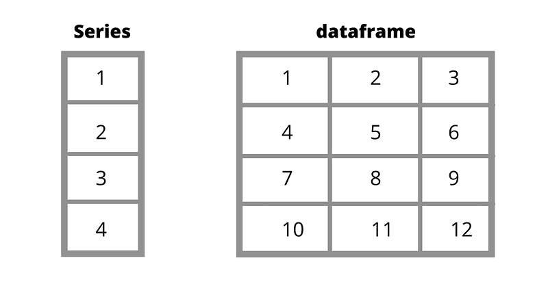
Pandas Series is a one-dimensional labeled array capable of holding data of any type (integer, string, float, python objects, etc.). Series in Pandas returns both values and indexes associated with it.

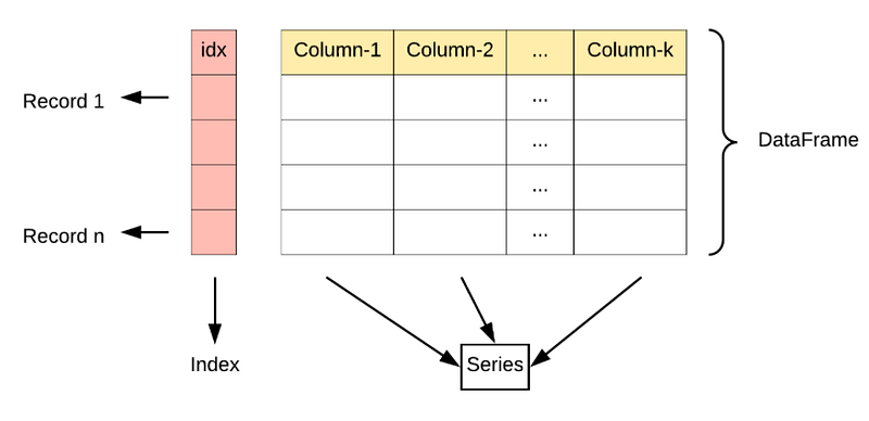
Pandas DataFrame is two-dimensional size-mutable, a heterogeneous tabular data structure with labeled axes (rows and columns). A Data frame is a two-dimensional data structure, i.e. data is aligned in a tabular fashion in rows and columns.

A Pandas Series is a one-dimensional array of indexed data. It can be created from a list or array as follows -

To create Pandas Series —

pd.Series(data, index=index)

Example -

s = pd.Series([1, 1.5, 1.75,])

Pandas DataFrame is an analog of a two-dimensional array with both flexible row indices and flexible column names.

To create Pandas DataFrame —

pd.DataFrame(data, index=index)

Example -

pd.DataFrame(Data, index=index)

A Pandas Index is an immutable array or as an ordered set

Example -

i = pd.Index([2, 3, 5, 7, 11])

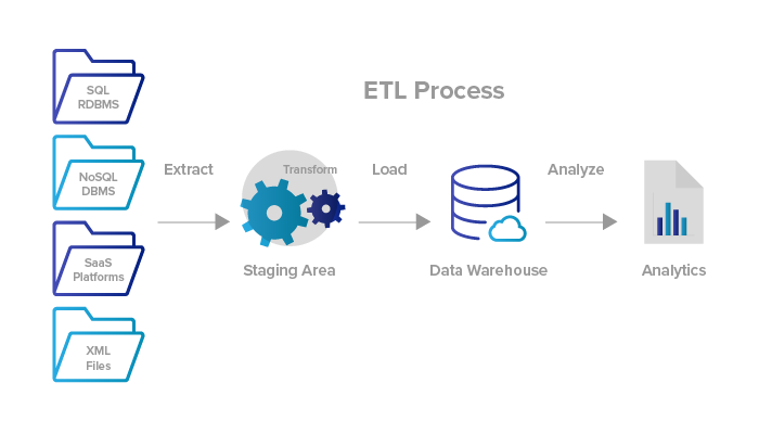
Data Processing

It’s a technique/process which involves conversion of data into usable and desired form. Data processing starts with data in its raw form and converts it into a more readable format ( image, graph, table, vector file, audio, charts etc)

Mega Compilation : Complete Tech Interview Series Roundup — Part 1

Three types of Data Processing : Manual data processing, Mechanical data processing and Electronic data processing

Various tools —

Calculation and Analysis tools — Excel and Calculators — tools that help in applying relevant formulas to process the whole data

Statistical Tools — SAS

Database tools — Oracle, MongoDb, Hadoop etc that help in processing large amounts of data

Data Cleaning

Data Cleaning is the process of correcting or removing incorrect, incomplete, or duplicate data within a given dataset. Proper data cleaning can make or break your project. Hence, data science professionals usually spend a very large portion of their time on Data Cleaning.

The golden rule is — Better data beats fancier algorithms

Ask Questions -

Completeness: Does the given data include all required information?

Validity: Does the given data correspond with business rules and/or restrictions?

Uniformity: Is the given data specified using consistent units of measurement?

Consistency: Is the given data consistent across your datasets?

Accuracy: Is the given data close to the true values?

Data Cleaning is an important process and it starts with removing unwanted samples/observations in the given dataset

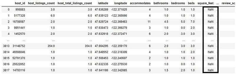
Missing Data

Missing data is the data that is not captured for a variable for the observation in question. If the missing values are not handled properly by the data science professional, then he may end up drawing an inaccurate inference about the data. Missing data reduces the statistical power of the analysis, which can distort the validity of the results.

Hence, it is very important to handle missing data because any statistical results based on a dataset with non-random missing values could be biased and lead to inaccurate results in the end

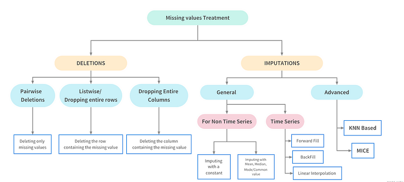
Ways to Handle Missing Values

Drop missing values

Ignore tuples with missing values

Imputation etc

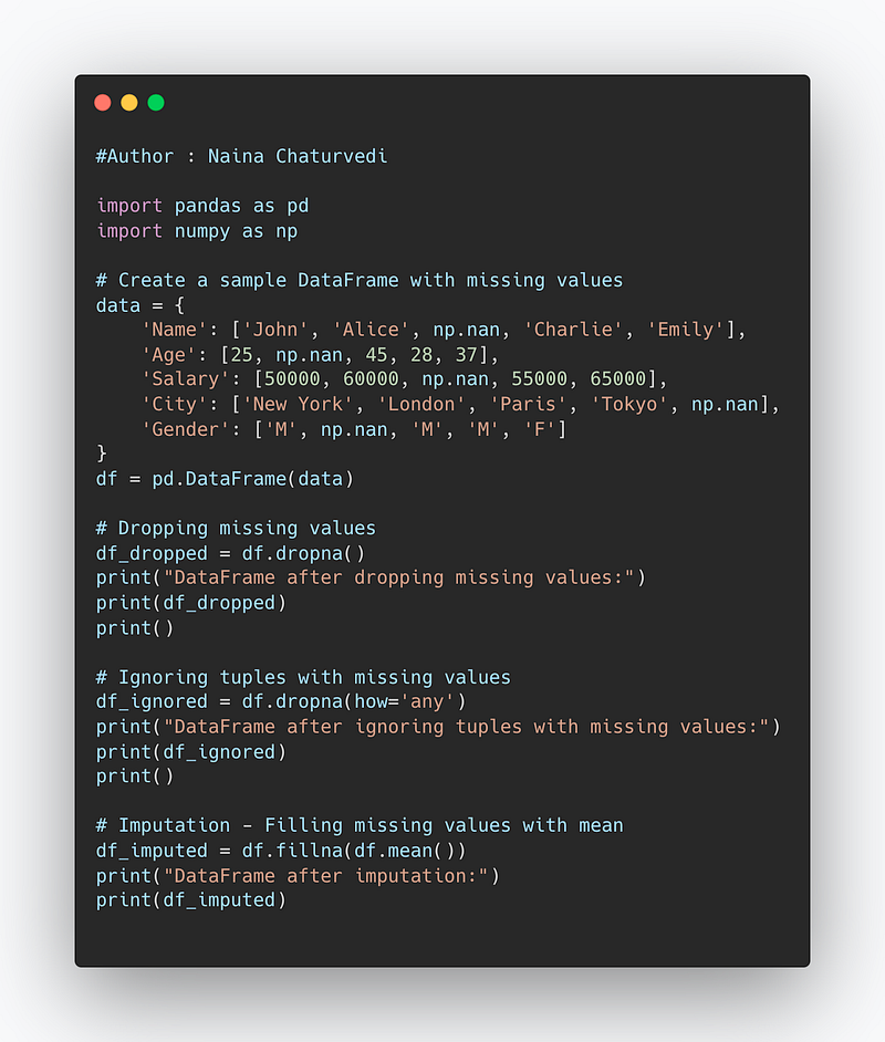
import pandas as pd
import numpy as np

# Create a sample DataFrame with missing values
data = {
    'Name': ['John', 'Alice', np.nan, 'Charlie', 'Emily'],
    'Age': [25, np.nan, 45, 28, 37],
    'Salary': [50000, 60000, np.nan, 55000, 65000],
    'City': ['New York', 'London', 'Paris', 'Tokyo', np.nan],
    'Gender': ['M', np.nan, 'M', 'M', 'F']
}
df = pd.DataFrame(data)

# Dropping missing values
df_dropped = df.dropna()
print("DataFrame after dropping missing values:")
print(df_dropped)
print()

# Ignoring tuples with missing values
df_ignored = df.dropna(how='any')
print("DataFrame after ignoring tuples with missing values:")
print(df_ignored)
print()

# Imputation - Filling missing values with mean
df_imputed = df.fillna(df.mean())
print("DataFrame after imputation:")
print(df_imputed)

Snippet —

Noisy Data

Noise unwanted/meaningless data items, features or records which don’t help in explaining the feature itself, or the relationship between feature & target. The occurrences of noisy data in data set can significantly impact prediction of any meaningful information and causes the algorithms to miss out patterns in the data. Noise in data set dramatically led to decreased classification accuracy and poor prediction results. It can be — certain anomalies in features & target, irrelevant/weak features and noisy records.

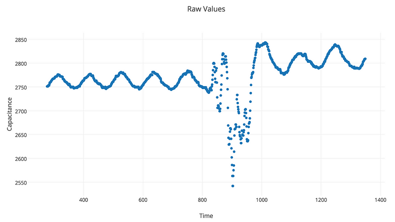
Therefore, it becomes important for any data scientist to take care as well as eliminate noise when applying any algorithm over a noisy data.

Techniques to handle Noisy data —

Binning

import pandas as pd
import numpy as np
from sklearn.preprocessing import KBinsDiscretizer

# Create a sample DataFrame
data = {
    'Age': [25, 32, 45, 28, 37, 50, 60, 70],
    'Income': [50000, 60000, 70000, 55000, 65000, 80000, 90000, 100000]
}
df = pd.DataFrame(data)

# Perform binning on 'Age' column
est = KBinsDiscretizer(n_bins=3, encode='ordinal', strategy='uniform')
df['Age_Bins'] = est.fit_transform(df[['Age']])

print("DataFrame after binning:")
print(df)

Regression

import pandas as pd
import numpy as np
from sklearn.linear_model import LinearRegression

# Create a sample DataFrame
data = {
    'Hours_Studied': [2, 4, 6, 8, 10],
    'Score': [60, 70, 80, 90, 95]
}
df = pd.DataFrame(data)

# Perform linear regression
X = df[['Hours_Studied']]
y = df['Score']
reg = LinearRegression().fit(X, y)

# Predict score for new hours studied
new_hours_studied = [[7]]
predicted_score = reg.predict(new_hours_studied)

print("Predicted Score:", predicted_score[0])

Clustering

import pandas as pd
import numpy as np
from sklearn.cluster import KMeans

# Create a sample DataFrame
data = {
    'X': [2, 2, 8, 5, 7, 6],
    'Y': [10, 5, 4, 8, 5, 2]
}
df = pd.DataFrame(data)

# Perform k-means clustering
kmeans = KMeans(n_clusters=2, random_state=0).fit(df)

# Get cluster labels for the data points
cluster_labels = kmeans.labels_

print("Cluster Labels:", cluster_labels)

Outlier Detection

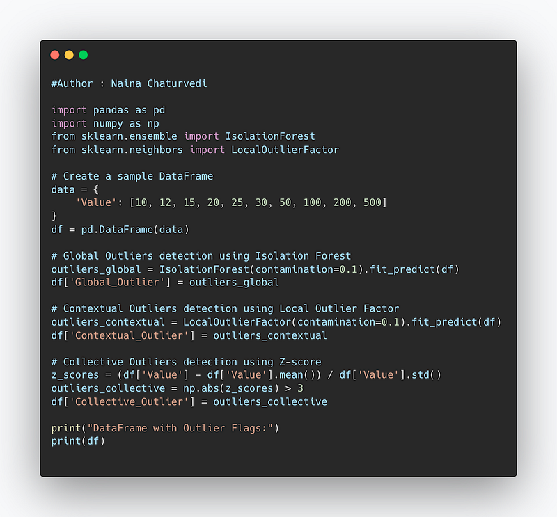
An outlier is an observation that diverges from an overall pattern on a sample. Outliers are extreme values that deviate from other observations on data , they may indicate a variability in a measurement, experimental errors. The presence of outliers in a classification or regression dataset can result in a poor fit and lower predictive modeling performance and can skew statistical measures and data distributions, providing a misleading representation of the underlying data and relationships. Outlier Detection is the technique of detecting and subsequently excluding outliers from a given set of data.

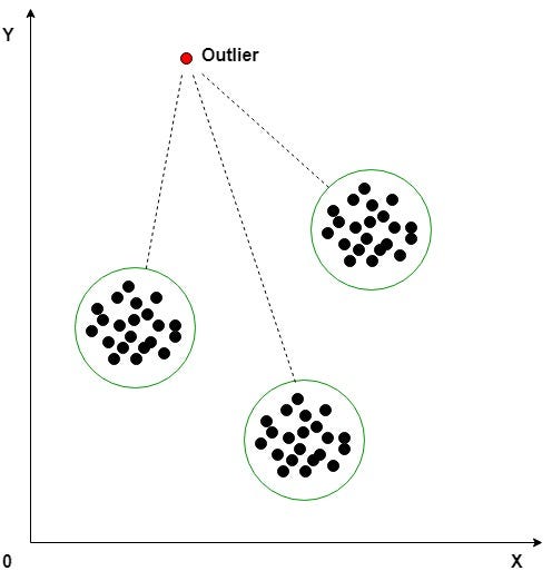
Types of Outliers —

Global Outliers : point value is far outside the entirety of the data set

Contextual Outliers : point value which significantly deviates from the rest of the data points in the same context

Collective Outliers : point value as a collection deviate significantly from the entire data set

import pandas as pd
import numpy as np
from sklearn.ensemble import IsolationForest
from sklearn.neighbors import LocalOutlierFactor

# Create a sample DataFrame
data = {
    'Value': [10, 12, 15, 20, 25, 30, 50, 100, 200, 500]
}
df = pd.DataFrame(data)

# Global Outliers detection using Isolation Forest
outliers_global = IsolationForest(contamination=0.1).fit_predict(df)
df['Global_Outlier'] = outliers_global

# Contextual Outliers detection using Local Outlier Factor
outliers_contextual = LocalOutlierFactor(contamination=0.1).fit_predict(df)
df['Contextual_Outlier'] = outliers_contextual

# Collective Outliers detection using Z-score
z_scores = (df['Value'] - df['Value'].mean()) / df['Value'].std()
outliers_collective = np.abs(z_scores) > 3
df['Collective_Outlier'] = outliers_collective

print("DataFrame with Outlier Flags:")
print(df)

Snippet —

One hot encoding

One hot encoding is used for treating categorical variables. One hot encoding creates new (binary) columns, indicating the presence of each possible value from the original data

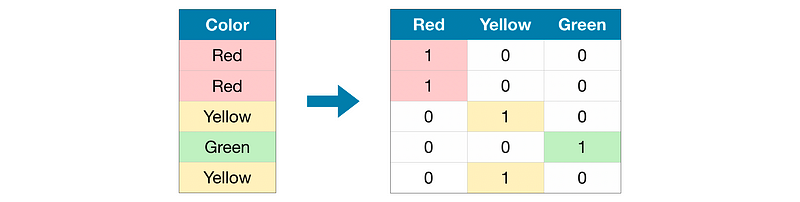
It simply creates additional features based on the number of unique values in the categorical feature

One hot encoder only takes numerical categorical values, hence any value of string type should be label encoded before one-hot encoded

One hot encoding makes our training data more useful and expressive, and it can be rescaled easily

import pandas as pd
from sklearn.preprocessing import OneHotEncoder

# Create a sample DataFrame
data = {
    'Color': ['Red', 'Blue', 'Green', 'Blue', 'Red', 'Green']
}
df = pd.DataFrame(data)

# Perform one-hot encoding
encoder = OneHotEncoder()
encoded_data = encoder.fit_transform(df[['Color']])
df_encoded = pd.DataFrame(encoded_data.toarray(), columns=encoder.categories_[0])

print("DataFrame after one-hot encoding:")
print(df_encoded)

Label Encoding

Label Encoding is used to handle categorical variables. In this technique, each label is assigned a unique integer based on alphabetical ordering.

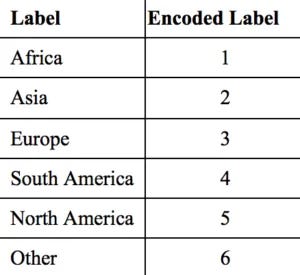
Sklearn provides a method for encoding the categories of categorical features into numeric values

Label encoder encodes labels with credit between 0 and n-1 classes where n is the number of diverse labels

It can be implemented using preprocessing module from sklearn package and them import LabelEncoder class as below:

import pandas as pd
from sklearn.preprocessing import LabelEncoder

# Create a sample DataFrame
data = {
    'Color': ['Red', 'Blue', 'Green', 'Blue', 'Red', 'Green']
}
df = pd.DataFrame(data)

# Perform label encoding
encoder = LabelEncoder()
df['Encoded_Color'] = encoder.fit_transform(df['Color'])

print("DataFrame after label encoding:")
print(df)

Pandas Series

Pandas Series is a one-dimensional labeled array capable of holding data of any type.

s = pd.Series([100,290,40,199,76])
s

Output —

0     100
1     290
2     40
3    199
4     76
dtype: int64

To check the type —

type(s)

Output —

pandas.core.series.Series

Series.axes attribute returns a list of row axis labels of the given Series object.

s.axes

Output —

[RangeIndex(start=0, stop=5, step=1)]

Checking the DataType of the Series

s.dtype

Output —

dtype('int64')

Series.size — Size attribute returns the number of elements in the underlying data for the given series objects.

s.size

Output —

5

ndim attribute returns the number of dimensions of the underlying data, by definition it is 1 for series objects.

s.ndim

Output —

1

Series.values attribute return Series as ndarray or ndarray-like depending on the dtype.

s.values

Output —

array([ 100,  290,  40, 199,  76], dtype=int64)

We can also specify our Indexes in Strings/Objects.

s1 = pd.Series([1,2,4,5,6],index = ["First","Zero","Second","Third","Fourth"])

Output —

First     1
Zero      2
Second    4
Third     5
Fourth    6
dtype: int64

If we are using the string based indexes and if we run sort_index() throughout the series, then it will arrange the Series elements on the basis of alphabetically.

s1.sort_index()

Output —

First     1
Fourth    6
Second    4
Third     5
Zero      2
dtype: int64

Creating Series with Dictionaries

ages = {'Andrew':31,"Kate":45,"Matthew":26,"Helen":19}
new_ages = pd.Series(ages)
new_ages

Output —

Andrew     31
Kate       45
Matthew    26
Helen      19
dtype: int64

If we only want to select a Particular elements from the dictionary then we can use index.

pd.Series(ages,index =["Andrew","Helen"])

Output —

Andrew    31
Helen     19
dtype: int64

Creating Pandas Series by Numpy Arrays

import numpy as np

We can also create series using numpy.

n_one = np.array([1,2,3,4])
pd.Series(n_one)

Output —

0    1
1    2
2    3
3    4
dtype: int32

Merging Two Series (Concat)

s1 = pd.Series([2,3,55,2,6,44]) 
s2 = pd.Series([42,32,34,2,1,4,42])
pd.concat([s1,s2])

Output —

0       2
1       3
2      55
3       2
4       6
5      44
0      42
1      32
2      34
3       2
4       1
5       4
6      42
dtype: int64

we can use selection and use different selectors to select specific elements from the Series.

l = pd.Series([11,12,13,14,15,16])
l[0:3]

Output —

0    11
1    12
2    13
dtype: int64

Pandas DataFrame

Creating a DataFrame

names = {"Names":["Allen","Rob","Harold","Amy"],"Age":[21,11,13,15]}

# Creating a DataFrame using a Dictionary.

new_dic = pd.DataFrame(names)
new_dic["Age"]

Output —

0    21
1    11
2    13
3    15
Name: Age, dtype: int64

We can also Assign Column name —

var = [10,30,20,89,48,40]
df = pd.DataFrame(var,columns = ["Variables"])

We can also create DataFrames from Numpy —

arr = np.random.randint(10,size = (5,2))
arr

Output —

array([[5, 0],
       [6, 3],
       [8, 0],
       [2, 2],
       [8, 0]])

We can assign them the columns name —

new_arr= pd.DataFrame(arr,columns = ["Var1","Var2"])

DataFrame.axes attribute access a group of rows and columns by label(s) or a boolean array in the given DataFrame.

new_arr.axes

Output —

[RangeIndex(start=0, stop=5, step=1), Index(['Var1', 'Var2'], dtype='object')]

To determine shape —

new_arr.shape

Output —

(5, 2)

Checking the Dimension of the DataFrame

new_arr.ndim

Output —

(5, 2)

Checking the total number of elements in the DataFrame

new_arr.size

Output —

10

Getting the Columns Names from the DataFrame

new_arr.columns

Output —

Index(['Var1', 'Var2'], dtype='object')

Index — The index (row labels) of the DataFrame. It basically tells us that how many rows our DataFrame has.

new_arr.index

Output —

RangeIndex(start=0, stop=5, step=1)

Values — DataFrame.values attribute return a Numpy representation of the given DataFrame.

new_arr.values

Output —

array([[5, 0],
       [6, 3],
       [8, 0],
       [2, 2],
       [8, 0]])

Accessing the rows of the DataFrame

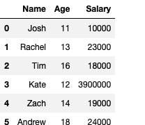
dfc = pd.DataFrame({"Name":["Josh","Rachel","Tim","Kate","Zach","Andrew"],"Age":[11,13,16,12,14,18],"Salary":[10000,23000,18000,3900000,19000,24000]})

Output —

dfc.Age

Output —

0    11
1    13
2    16
3    12
4    14
5    18
Name: Age, dtype: int64

Now if we want to access the rows specific —

dfc["Age"][3]

Output —

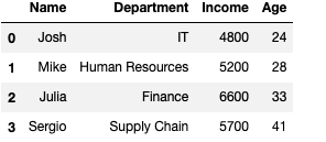
12

Filtering

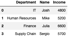
employees = pd.DataFrame({"Name":["Josh","Mike","Julia","Sergio"],
                          "Department":["IT","Human Resources","Finance","Supply Chain"],"Income":[4800,5200,6600,5700],
"Age":[24,28,33,41]})
employees

Output —

Now, if want to check according to Specific Department —

employees["Department"] == "IT"

Output —

0     True
1    False
2    False
3    False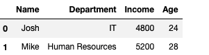
Name: Department, dtype: bool

We can also use the loc[] Operator and it gives us the flexibility to choose from between various Departments

employees.loc[employees["Department"] == "IT","Name"]

Output —

0    Josh
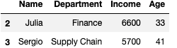
Name: Name, dtype: object

Now if we want to know the salary of the employees based on some arithmetic conditions

employees[employees["Income"] >5500]

Output —

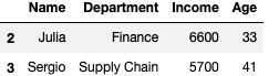
employees[(employees["Age"]>30) | (employees["Department"] == "HR")]

Output —

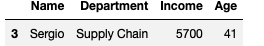
To get opposite of a filter use ~(Tilde) sign —

employees[~(employees["Age"]<35)]

Output —

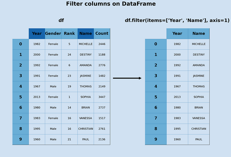
Filtering with Filter () Function —

employees.filter(items=["Department","Name","Income"])

Output —

Adding Rows — append()

employees.append({"Name":"Romeo"},ignore_index=True)

Output —

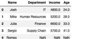
It adds automatically to the end of dataframe. But we need to add all values, otherwise it gives nan.

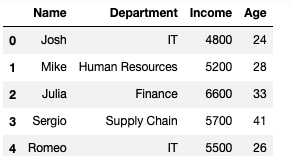
employees.append({"Name":"Romeo","Age":26,"Department":"IT","Income":5500},ignore_index=True)

Output —

Removing Rows —

employees.drop(employees[employees["Age"]>30].index)

Output —

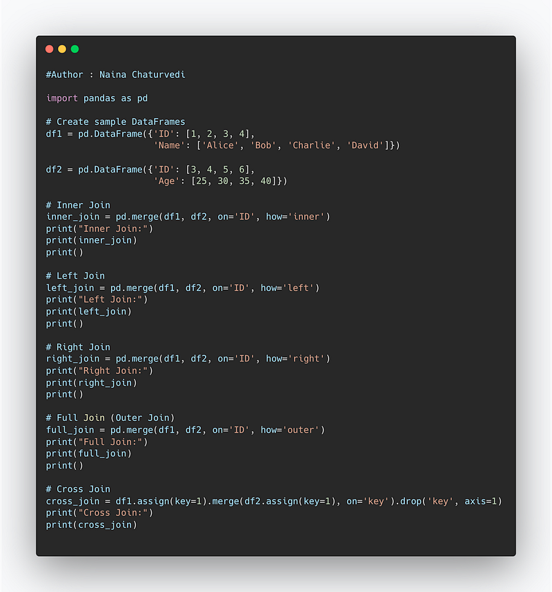
Joins

Used to merge DataFrames.

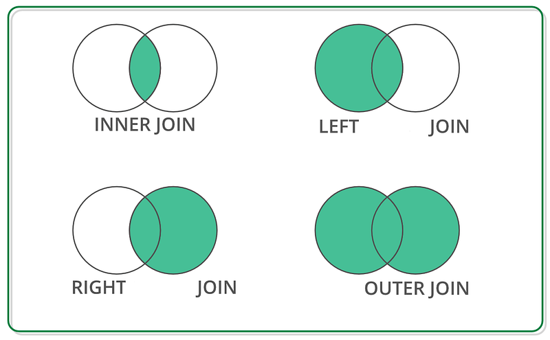
Inner Join :- Returns records that have matching values in both tables.

Left Join :- Returns all the rows from the left table that are specified in the left outer join clause.

Right Join :- Returns all records from the right table, and the matched records from the left table.

Full Join :- Returns all records when there is a match in either left or right table.

Cross Join :- Returns all possible combinations of rows from two tables.

import pandas as pd

# Create sample DataFrames
df1 = pd.DataFrame({'ID': [1, 2, 3, 4],
                    'Name': ['Alice', 'Bob', 'Charlie', 'David']})

df2 = pd.DataFrame({'ID': [3, 4, 5, 6],
                    'Age': [25, 30, 35, 40]})

# Inner Join
inner_join = pd.merge(df1, df2, on='ID', how='inner')
print("Inner Join:")
print(inner_join)
print()

# Left Join
left_join = pd.merge(df1, df2, on='ID', how='left')
print("Left Join:")
print(left_join)
print()

# Right Join
right_join = pd.merge(df1, df2, on='ID', how='right')
print("Right Join:")
print(right_join)
print()

# Full Join (Outer Join)
full_join = pd.merge(df1, df2, on='ID', how='outer')
print("Full Join:")
print(full_join)
print()

# Cross Join
cross_join = df1.assign(key=1).merge(df2.assign(key=1), on='key').drop('key', axis=1)
print("Cross Join:")
print(cross_join)

Snippet —

Inner Join —

c1 = pd.DataFrame({"Name":['Amy','Allen','Alice','Anderson','Amanda'],"Age":[21,22,26,29,32],"Roll Number":[12,19,29,10,8]})c2 =pd.DataFrame({"Marks":[90,89,82,98,85],"Roll Number":[1,90,29,48,67]})

Use join= “inner”

pd.concat([c1,c2],join= "inner")

Full Join — Returns all records when there is a match in either left or right table.

pd.concat([c1,c2],join = "outer",ignore_index=True)

Left Join — Returns all the rows from the left table that are specified in the left outer join clause, not just the rows in which the columns match.

pd.merge(c1,c2,how ="left")

Right Join :- Returns all records from the right table, and the matched records from the left table.

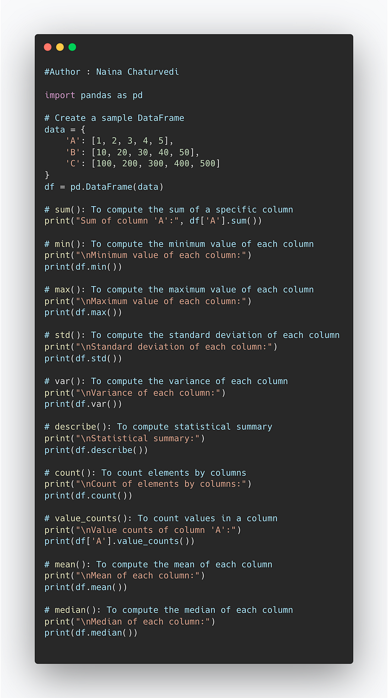
pd.merge(c1,c2,how ="right")

Aggregate Functions

• sum() : To compute the sum of a specific Column.
• min() : To compute minimum value of each Column
• max() : To compute maximum value of each Column
• std() : To compute Standard Deviation of each column

• var() : To Compute variance of each column
• describe() : To compute statistical summary
• count() : To count elements by elements.
• value_count() : To count value in column
• mean() : To Compute Mean of each column
• median() : Compute Median of each column

Code Implementation —

import pandas as pd

# Create a sample DataFrame
data = {
    'A': [1, 2, 3, 4, 5],
    'B': [10, 20, 30, 40, 50],
    'C': [100, 200, 300, 400, 500]
}
df = pd.DataFrame(data)

# sum(): To compute the sum of a specific column
print("Sum of column 'A':", df['A'].sum())

# min(): To compute the minimum value of each column
print("\nMinimum value of each column:")
print(df.min())

# max(): To compute the maximum value of each column
print("\nMaximum value of each column:")
print(df.max())

# std(): To compute the standard deviation of each column
print("\nStandard deviation of each column:")
print(df.std())

# var(): To compute the variance of each column
print("\nVariance of each column:")
print(df.var())

# describe(): To compute statistical summary
print("\nStatistical summary:")
print(df.describe())

# count(): To count elements by columns
print("\nCount of elements by columns:")
print(df.count())

# value_counts(): To count values in a column
print("\nValue counts of column 'A':")
print(df['A'].value_counts())

# mean(): To compute the mean of each column
print("\nMean of each column:")
print(df.mean())

# median(): To compute the median of each column
print("\nMedian of each column:")
print(df.median())

Implementation —

#Create dataframe eemployee

employees = pd.DataFrame({"Name":["A","B","C","D","E","F"],"Department":["Finance","Human Resources","Finance","Supply Chain","IT","Marketing"],"Income":[3000,6000,8000,5500,2300,4400],"Age":[20,25,30,40,21,42]})

employees.count()

employees["Department"].value_counts()

employees.mean()

employees["Income"].sum()

employees["Age"].min()

employees["Age"].max()

employees["Age"].std()

employees.var()

employees.describe()

Snippet —

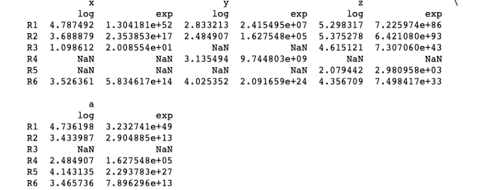
Transforming Data Frames

Pandas Transform helps in creating a DataFrame with transformed values and has the same axis length as its own.

Syntax: df.transform(function, axis=0, *args, **kwargs)

where function — Function for transforming the data axis : 0 for rows and 1 for column *args : Positional arguments **kwargs : Keyword arguments

Implementation —

import pandas as pd
  
df = pd.DataFrame({"x":[120, 40, 3, None, None,34], 
                   "y":[17, 12, None, 23, None,56], 
                   "z":[200, 216, 101, None, 8,78], 
                   "a":[114, 31, None, 12, 63,32]}) 
  
index_ = ['R1', 'R2', 'R3', 'R4', 'R5','R6']df.index = index_res = df.transform(func = ['log', 'exp'])
  
print(res)

Output —

Grouping

• Split Object
• Applying groupby Function

employees = pd.DataFrame({"Name":["A","B","C","D","E","F"], "Department":["Finance","Human Resources","Finance","Supply Chain","IT","Marketing"], "Income":[3000,6000,8000,5500,2300,4400], "Age":[20,25,30,40,21,42]})

emp = employees.groupby("Department")
employees.groupby("Department").mean()

Hierarchical indexing

Hierarchical indexing is the technique in which we set more than one column name as the index. set_index() function is used for when doing hierarchical indexing.

Implementation —

index = pd.MultiIndex.from_product([[2020, 2021], [3, 4]],
                                   names=['year', 'round'])
columns = pd.MultiIndex.from_product([['Claire', 'Kassi', 'Suer'], ['Engg', 'Maths']],
                                     names=['subject', 'class'])data = np.round(np.random.randn(4, 6), 1)
data[:, ::3] *= 5
data += 19df = pd.DataFrame(data, index=index, columns=columns)

Indexing data frames

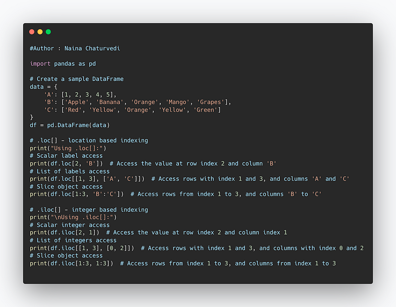
Indexing means to selecting all/particular rows and columns of data from a DataFrame. In pandas it can be done using three constructs —

.loc() : location based

It has methods like scalar label, list of labels, slice object etc

.iloc() : Interger based

.ix() : Both integer and location based

import pandas as pd

# Create a sample DataFrame
data = {
    'A': [1, 2, 3, 4, 5],
    'B': ['Apple', 'Banana', 'Orange', 'Mango', 'Grapes'],
    'C': ['Red', 'Yellow', 'Orange', 'Yellow', 'Green']
}
df = pd.DataFrame(data)

# .loc[] - location based indexing
print("Using .loc[]:")
# Scalar label access
print(df.loc[2, 'B'])  # Access the value at row index 2 and column 'B'
# List of labels access
print(df.loc[[1, 3], ['A', 'C']])  # Access rows with index 1 and 3, and columns 'A' and 'C'
# Slice object access
print(df.loc[1:3, 'B':'C'])  # Access rows from index 1 to 3, and columns 'B' to 'C'

# .iloc[] - integer based indexing
print("\nUsing .iloc[]:")
# Scalar integer access
print(df.iloc[2, 1])  # Access the value at row index 2 and column index 1
# List of integers access
print(df.iloc[[1, 3], [0, 2]])  # Access rows with index 1 and 3, and columns with index 0 and 2
# Slice object access
print(df.iloc[1:3, 1:3])  # Access rows from index 1 to 3, and columns from index 1 to 3

Implementation —

import pandas as pd
import numpy as npdf = pd.DataFrame(np.random.randn(4, 3),
index = ['a','b','c','d'], columns = ['X', 'Y', 'Z'])
print (df.loc['c']> 0)

Output —

X    False
Y     True
Z     True
Name: c, dtype: bool

Implementation —

import pandas as pd
import numpy as npdf = pd.DataFrame(np.random.randn(8, 4), columns = ['X', 'Y', 'Z', 'A'])# Slicing through list of values
print (df.iloc[[1, 2, 3], [1, 3]])

Output —

Y         A
1  0.566221  1.934828
2 -1.814986 -1.829436
3 -0.264360  0.860286

Snippet —

That’s it for now.

Find Day 14 Below —

Let me know if you have questions in the comment section below. Subscribe/ Follow, Like/Clap as it would encourage me to write more in my free time

Stay Tuned!!

Read more —

All the Complete System Design Series Parts —

1. System design basics

2. Horizontal and vertical scaling

3. Load balancing and Message queues

4. High level design and low level design, Consistent Hashing, Monolithic and Microservices architecture

5. Caching, Indexing, Proxies

6. Networking, How Browsers work, Content Network Delivery ( CDN)

7. Database Sharding, CAP Theorem, Database schema Design

8. Concurrency, API, Components + OOP + Abstraction

9. Estimation and Planning, Performance

10. Map Reduce, Patterns and Microservices

11. SQL vs NoSQL and Cloud

12. Most Popular System Design Questions

Github —

Keep learning and coding ;)

Day 5 coming soon!

For Python Projects —

For complete 60 days of Data Science and ML : Day 1 — Day 60 : Quick Recap of 60 days of Data Science and ML

Follow for more updates. Stay tuned and keep coding! Disclosure: Some of the links are affiliates.

For other projects, tune to —

Build Machine Learning Pipelines( With Code)

Recurrent Neural Network with Keras

Clustering Geolocation Data in Python using DBSCAN and K-Means

Facial Expression Recognition using Keras

Hyperparameter Tuning with Keras Tuner

Custom Layers in Keras