23 Data Science Techniques You Should Know!

Save your precious time by using these hacks

Data scientists are high in demand. The job of a data scientist is not easy, so it’s important to know a few data science hacks that can save your precious time and make your life simpler. In this post, I’m going to cover 23 data science hacks that I have used.

Projects Videos —

All the projects, data structures, SQL, algorithms, system design, Data Science and ML , Data Analytics, Data Engineering, , Implemented Data Science and ML projects, Implemented Data Engineering Projects, Implemented Deep Learning Projects, Implemented Machine Learning Ops Projects, Implemented Time Series Analysis and Forecasting Projects, Implemented Applied Machine Learning Projects, Implemented Tensorflow and Keras Projects, Implemented PyTorch Projects, Implemented Scikit Learn Projects, Implemented Big Data Projects, Implemented Cloud Machine Learning Projects, Implemented Neural Networks Projects, Implemented OpenCV Projects,Complete ML Research Papers Summarized, Implemented Data Analytics projects, Implemented Data Visualization Projects, Implemented Data Mining Projects, Implemented Natural Leaning Processing Projects, MLOps and Deep Learning, Applied Machine Learning with Projects Series, PyTorch with Projects Series, Tensorflow and Keras with Projects Series, Scikit Learn Series with Projects, Time Series Analysis and Forecasting with Projects Series, ML System Design Case Studies Series videos will be published on our youtube channel ( just launched).

Subscribe today!

Here are some essential data science techniques that every data scientist should know:

1. Data Exploration and Visualization: Understanding your data is critical for building effective models. This includes exploring the distribution of variables, identifying outliers and missing values, and creating visualizations to help identify patterns and relationships in the data.
2. Data Preprocessing: Preprocessing is an important step in preparing your data for analysis and modeling. This may include imputing missing values, transforming variables, and scaling data to ensure all variables are on a similar scale.
3. Feature Engineering: Feature engineering involves creating new variables or transforming existing variables to improve the performance of a model. This can include creating interactions between variables, binning variables, or extracting features from text data.
4. Model Selection: There are many algorithms to choose from when building a model, and selecting the best algorithm depends on the specific problem you are trying to solve and the properties of your data. Techniques such as cross-validation can be used to compare the performance of different algorithms and select the best one.
5. Model Evaluation: Once you have built a model, it’s important to evaluate its performance to ensure it generalizes well to new data. Common metrics for evaluating the performance of a model include accuracy, precision, recall, and F1 score.
6. Hyperparameter tuning: Many machine learning algorithms have hyperparameters that control their behavior. Fine-tuning these hyperparameters can significantly improve the performance of a model. Common techniques for hyperparameter tuning include grid search and random search.
7. Ensemble Methods: Ensemble methods are techniques that combine the predictions of multiple models to produce a single, more accurate prediction. Common ensemble methods include bagging, random forests, and boosting.

1. Image Augmentation:

Image Augmentation is a very powerful technique that is used to create new and different images from the existing images. It is used to address issues associated with limited data in machine learning.

Import all the necessary libraries :

# importing all the required libraries
%matplotlib inline
import skimage.io as io
from skimage.transform import rotate
import numpy as np
import matplotlib.pyplot as plt

Read Image :

img= io.imread('/Users/priyeshkucchu/Desktop/image.jpeg')

Define Augment function :

def augment_img(img):
    fig,ax = plt.subplots(nrows=1,ncols=5,figsize=(22,12))
    ax[0].imshow(img)
    ax[0].axis('off')
    ax[1].imshow(rotate(img, angle=45, mode = 'wrap'))
    ax[1].axis('off')
    ax[2].imshow(np.fliplr(img))
    ax[2].axis('off')
    ax[3].imshow(np.flipud(img))
    ax[3].axis('off')
    ax[4].imshow(np.rot90(img))
    ax[4].axis('off')       
augment_img(img)

Highly Recommended Data Science and Machine Learning Courses that you MUST take ( with certificate) —

Complete Data Scientist

Complete Data Analyst

Complete Data Engineering

Complete Machine Learning Engineer

Complete Deep Learning

Complete Natural Language Processing

Complete Self Driving Car Engineer

2. Pandas Boolean Indexing

It’s a type of indexing method in which we can select subsets of data based on the actual values of the data in the DataFrame using a boolean vector to filter the data.

Import necessary libraries

import pandas as pd

Load Data

ytdata= pd.read_csv('/Users/priyeshkucchu/Desktop/USvideos.csv')

Boolean Indexing — Show only those rows where category_id is 24 and no of likes is greater than 12000

ytdata.loc[(ytdata['category_id']==24)& (ytdata['likes']>12000),\["category_id","likes"]].head()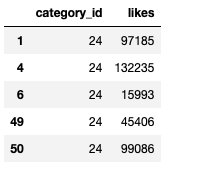

Some of the other best Series —

60 days of Data Science and ML Series with projects

How to solve any System Design Question ( approach that you can take)?

30 Days of Natural Language Processing ( NLP) Series

30 days of Machine Learning Ops

30 days of Data Structures and Algorithms and System Design Simplified

60 Days of Deep Learning with Projects Series

30 days of Data Engineering with projects Series

Data Science and Machine Learning Research ( papers) Simplified **

100 days : Your Data Science and Machine Learning Degree Series with projects

23 Data Science Techniques You Should Know

Tech Interview Series — Curated List of coding questions

Complete System Design with most popular Questions Series

Complete Data Visualization and Pre-processing Series with projects

Complete Python Series with Projects

Complete Advanced Python Series with Projects

Kaggle Best Notebooks that will teach you the most

Complete Developers Guide to Git

Exceptional Github Repos — Part 1

Exceptional Github Repos — Part 2

All the Data Science and Machine Learning Resources

210 Machine Learning Projects

Tech Newsletter —

If you are interested, you can join my newsletter through which I send tech interview tips, techniques, patterns, hacks — Software Development, ML, Data Science, Startups and Technology projects to more than 30K readers. You can subscribe to Tech Brew :

3. Pandas Pivot Table

In Pandas, the pivot table function takes a data frame as input and performs grouped operations that provide a multidimensional summarization of the data.

Import necessary libraries :

import pandas as pd
import numpy as np

Load Data :

loan = pd.read_csv('/Users/priyeshkucchu/Desktop/loan_train.csv', \ index_col = 'Loan_ID')

Show data :

loan.head()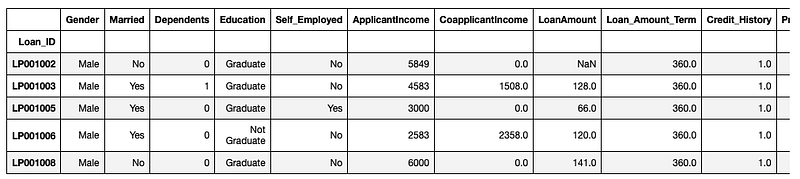

Pivot Table :

pivot = loan.pivot_table(values = ['LoanAmount'],index = ['Gender', \'Married','Dependents', 'Self_Employed'], aggfunc = np.median)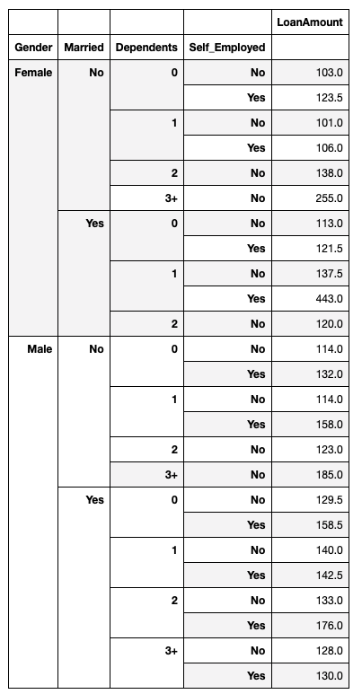

4. Pandas Apply

In Pandas, the .apply() function helps to segregate data based on the conditions as defined by the user.

Import necessary libraries

import pandas as pd

Load Data

ytdata= pd.read_csv('/Users/priyeshkucchu/Desktop/USvideos.csv')

Function Missing Values —

def missing_values(x):
    return sum(x.isnull())

For missing values in the columns —

print(" Missing values in each column :")
ytdata.apply(missing_values,axis=0)

Output —

Missing values in each column :

video_id                    0
trending_date               0
title                       0
channel_title               0
category_id                 0
publish_time                0
tags                        0
views                       0
likes                       0
dislikes                    0
comment_count               0
thumbnail_link              0
comments_disabled           0
ratings_disabled            0
video_error_or_removed      0
description               502
dtype: int64

For missing values in the rows —

print(" Missing values in each row :")
ytdata.apply(missing_values,axis=1).head()

Output —

Missing values in each row :

0    0
1    0
2    0
3    0
4    0
dtype: int64

5. Pandas Count

In pandas, the count function helps in counting Non-NA cells for each column or row.

Import necessary libraries :

import pandas as pd

Load Data :

ytdata= pd.read_csv('/Users/priyeshkucchu/Desktop/USvideos.csv')

Count no of data points in each column :

ytdata.count(axis=0)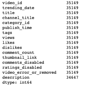

Count no. of null data points in the Description column

ytdata.description.isnull().value_counts()

6. Pandas Crosstab

In Pandas, this function is used to compute a simple cross-tabulation of two or more factors.

Import necessary libraries :

import pandas as pd

Load Data :

data = pd.read_csv('/Users/priyeshkucchu/Desktop/loan_train.csv',\ index_col = 'Loan_ID')

Cross tab between Credit History and Self Employed columns in the loan data :

pd.crosstab(data["Credit_History"],data["Self_Employed"],\
margins=True, normalize = False)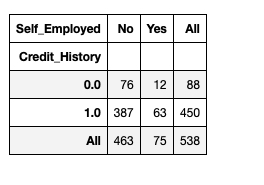

7. Pandas str.split

In Pandas, str.split function is used to provide a method to split string around a passed separator or a delimiter.

Import necessary libraries :

import pandas as pd

Create a Data Frame :

df = pd.DataFrame({'Person_name':['Naina Chaturvedi', 'Alvaro Morte', 'Alex Pina', 'Steve Jobs']})
df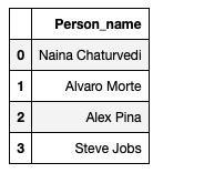

Extract First and Last Names:

df['first_name'] = df['Person_name'].str.split(' ',expand = True)[0]
df['last_name'] = df['Person_name'].str.split(' ', expand = True)[1]

df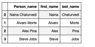

8. Extract E-mail from text

Import the necessary libraries and initialize the text :

import re

Enquiries_text = 'For any enquiries or feedback related to our product,\service, marketing promotions or other general support \ matters. [email protected]’'

Extract email using Regular Expression :

re.findall(r"([\w.-]+@[\w.-]+)", Enquiries_text)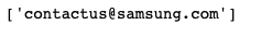

9. Pandas melt

In pandas, melt function is used to reshape the data frame to a longer form.

Import necessary libraries :

import pandas as pd

Create a Data Frame :

df = pd.DataFrame({'Person_Name': {0: 'Naina', 1: 'Alex', 2: \'Avarto'}, 'CourseName': {0: 'Masters', 1: 'Graduate', 2: \'Graduate'}, 'Age': {0: 27, 1: 20, 2: 22}})

Melt two data frames :

m1= pd.melt(df, id_vars =['Person_Name'], value_vars =['CourseName', 'Age'])
m1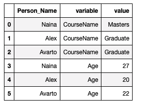

m2= pd.melt(df, id_vars =['Person_Name'], value_vars =['Age'])
m2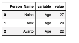

10. Extract Continuous and categorical data

Import necessary libraries :

import pandas as pd

Load Data :

Loan_data = pd.read_csv('/Users/priyeshkucchu/Desktop/loan_train.csv')
Loan_data.shape

Output: (614, 13)

Check data types of columns :

Loan_data.dtypes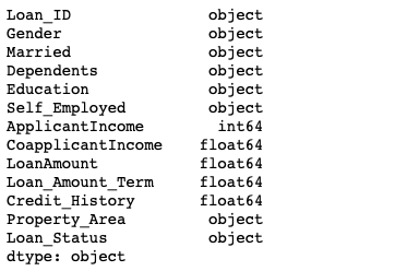

Extract columns containing only categorical data:

categorical_variables = Loan_data.select_dtypes("object").head()
categorical_variables.head()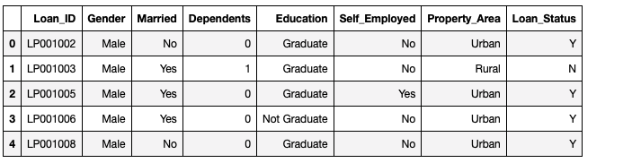

Extract columns containing only integer data:

integer_variables = Loan_data.select_dtypes("int64")
integer_variables.head()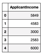

Extract columns containing only numerical data:

numeric_variables = Loan_data.select_dtypes("number")
numeric_variables.head()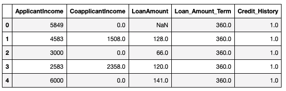

11. Pandas Eval function for efficient operations

The eval() function in Pandas uses string expressions to efficiently compute operations using a Data Frame.

Import necessary libraries :

import pandas as pd
import numpy as np

Initialize no_rows, no_cols:

no_rows, no_cols = 100000, 100
r = np.random.RandomState(50)
df1, df2, df3, df4 = (pd.DataFrame(r.rand(no_rows, no_cols))
                      for i in range(4))

Without Eval function

%timeit df1 + df2 * df3 - df4

With Eval function — The eval() version of this expression is about 50% faster and uses much less memory

%timeit pd.eval('df1 + df2 * df3 - df4')

12. Pandas Unique

In pandas, using unique function values that are unique are returned in order of appearance.

Import necessary libraries :

import pandas as pd
import numpy as np

Load Data :

crime_data = pd.read_csv("/Users/priyeshkucchu/Desktop/crime.csv",\ engine='python')

Show data :

crime_data.head()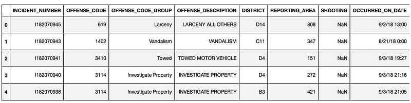

Show Unique values in the District Codes Column:

crime_data["DISTRICT"].unique()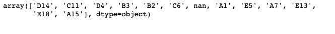

13. Ipython Interactive Shell

Import necessary libraries :

from IPython.core.interactiveshell import InteractiveShell
InteractiveShell.ast_node_interactivity = "all"
import pandas as pd

Load Data :

data = pd.read_csv('/Users/priyeshkucchu/Desktop/loan_train.csv')

Run commands simultaneously:

data.shape
data.head()
data.dtypes
data.info()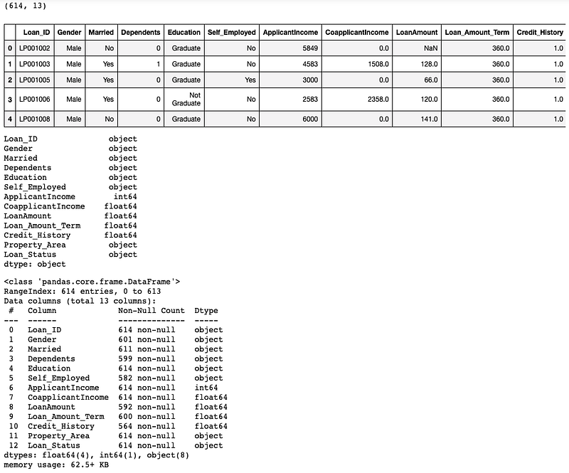

14. Pandas Merge

In pandas, the merge function is used to join two datasets together based on common columns between them.

Import necessary libraries :

import pandas as pd

Initialize Data Frames :

df1 = pd.DataFrame({'Left_key': ['Naina', 'Avarto', 'Alex', \'Naina'],'value': [1, 2, 3, 5]})
df2 = pd.DataFrame({'Right_key': ['Naina', 'Avarto', 'Alex', \'Naina'],'value': [5, 6, 7, 8]})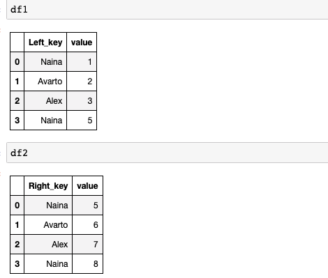

Merge the data frames :

df1.merge(df2, left_on='Left_key', right_on='Right_key', \
suffixes=('_Left', '_Right'))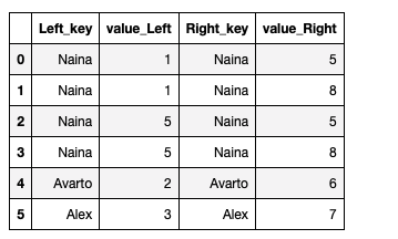

15. Parse dates in read_csv() to change data type to DateTime

Import necessary libraries :

import pandas as pd

Load Data and print the data types of crime data columns:

crime_data = pd.read_csv("/Users/priyeshkucchu/Desktop/crime.csv", \ engine='python')
crime_data.dtypes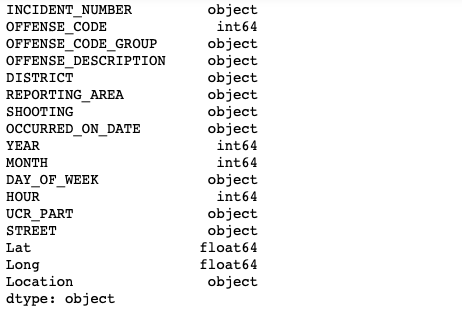

Parse Dates in read_csv():

crime_data = pd.read_csv("/Users/priyeshkucchu/Desktop/crime.csv", engine='python',parse_dates = ["OCCURRED_ON_DATE"])
crime_data.dtypes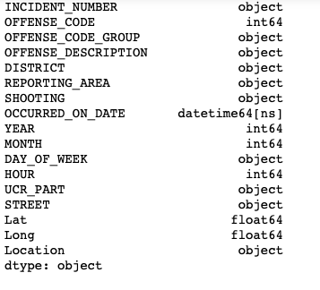

16. Date Parser

Import necessary libraries :

import datetime
import dateutil.parser

Parse Dates:

input_date = '04th Dec 2020'
parsed_date = dateutil.parser.parse(input_date)

Output date in the designated format :

op_date = datetime.datetime.strftime(parsed_date, '%Y-%m-%d')

print(op_date)

17. Invert a Dictionary

Create a dictionary :

l_dict = {'Person_Name':'Naina',
           'Age' : 27,
           'Profession' : 'Software Engineer'
           }

Original Dictionary :

Invert dictionary :

invert_dict = {values:keys for keys,values in l_dict.items()}
invert_dict

18. Pretty Dictionaries

Create a dictionary :

l_dict = {'Student_ID': 4,'Student_name' : 'Naina', 'Class_Name': '12th' ,'Student_marks' : {'maths' : 92,
                            'science' : 95,
                            'computer science' : 100,
                            'English' : 91}
          }

Original Dictionary :

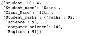
Pretty dictionary using pprint:

import pprint
pprint.pprint(l_dict)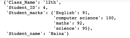

19. Convert List of list to list

Import necessary libraries:

import itertools

Create a list :

nested_list = [['Naina'], ['Alex', 'Rhody'], ['Sharron', 'Avarto', \'Grace']]
nested_list

Convert the list to list :

converted_list = list(itertools.chain.from_iterable(nested_list))

print(converted_list)

20. Removing Emojis from Text

Emoji_text = 'For example, 🤓🏃‍🏢 could mean “Iam running to work.”'
final_text=Emoji_text.encode('ascii', 'ignore').decode('ascii')

print("Raw tweet with Emoji:",Emoji_text)  
print("Final tweet withput Emoji:",final_text)

21. Apply Pandas Operations in Parallel

It’s used to distribute your pandas computations over all available CPUs on your computer to get a significant increase in the speed.

Install pandarallel :

!pip install pandarallel

Import necessary libraries:

%load_ext autoreload
%autoreload 2
import pandas as pd
import time
from pandarallel import pandarallel
import math
import numpy as np
import random
from tqdm._tqdm_notebook import tqdm_notebook
tqdm_notebook.pandas()

Initialize pandarallel :

pandarallel.initialize(progress_bar=True)

Dataframe:

df = pd.DataFrame({
    'A' : [random.randint(8,15) for i in range(1,100000) ],
    'B' : [random.randint(10,20) for i in range(1,100000) ]
})

Trigono function:

def trigono(x):
    return math.sin(x.A**2) + math.sin(x.B**2) + math.tan(x.A**2)

Without parallelization:

%%time
first = df.progress_apply(trigono, axis=1)

With parallelization:

%%time
first_parallel = df.parallel_apply(trigono, axis=1)

22. Pandas Cut and qcut

In Pandas,

cut command creates equispaced bins but the frequency of samples is unequal in each bin

qcut command creates unequal size bins but the frequency of samples is equal in each bin.

Import necessary Libraries:

import pandas as pd
import numpy as np

Dataframe:

df_rollno = pd.DataFrame({'Roll No': np.random.randint(20, 55, 10)})
df_rollno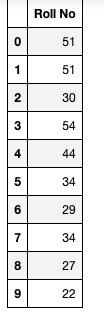

Using Pandas cut function :

df_rollno['roll_no_bins'] = pd.cut(x=df_rollno['Roll No'], bins=[20, 40, 50, 60])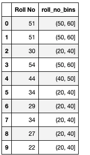

Using Pandas qcut function:

pd.qcut(df_rollno['Roll No'], q=6)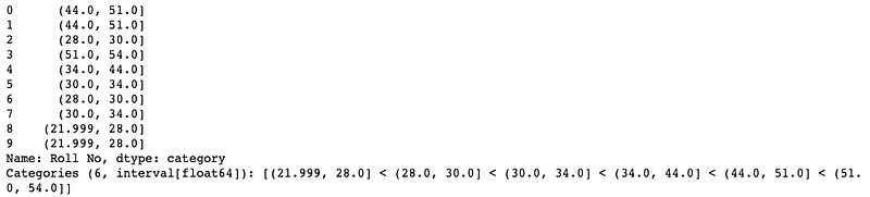

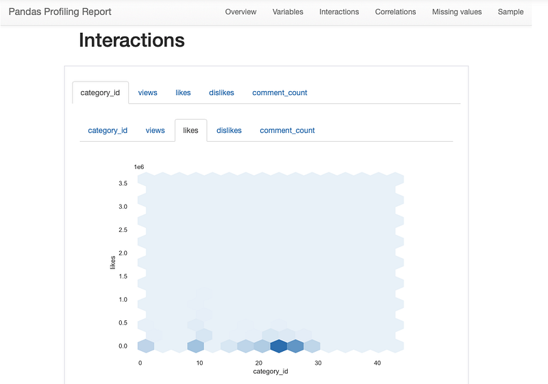
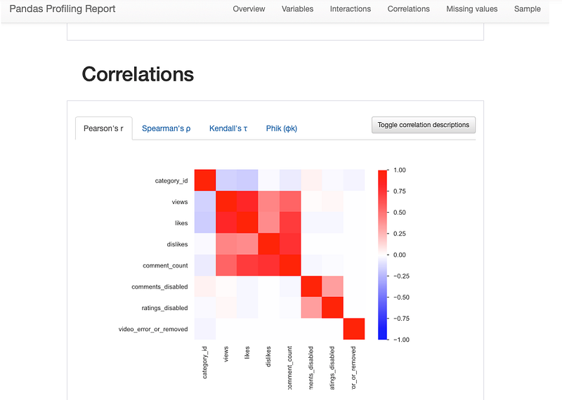
23. Pandas Profiling

It’s used to generates profile reports from a pandas DataFrame or data sheet.

Install Pandas Profiling:

pip install pandas-profiling

Import necessary libraries:

import pandas as pd
import pandas_profiling

Load Data:

Youtube_data = pd.read_csv('/Users/priyeshkucchu/Desktop/USvideos.csv')

Generate Profiling report:

profiling_report = pandas_profiling.ProfileReport(Youtube_data)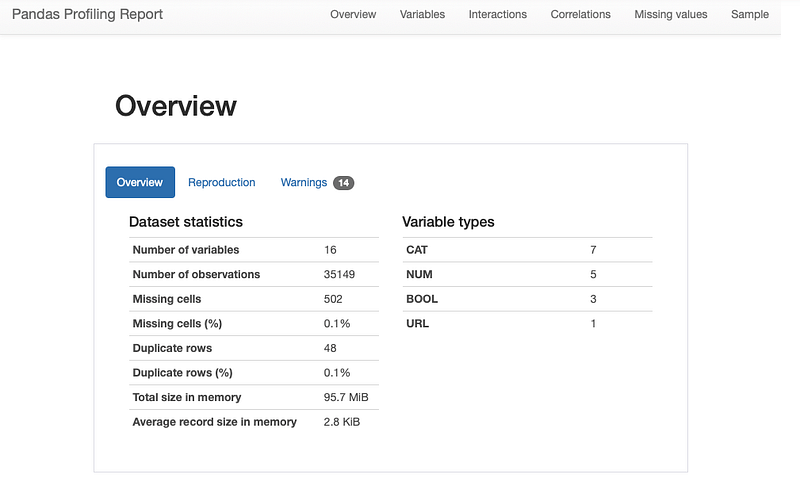

All the Complete System Design Series Parts —

1. System design basics

2. Horizontal and vertical scaling

3. Load balancing and Message queues

4. High level design and low level design, Consistent Hashing, Monolithic and Microservices architecture

5. Caching, Indexing, Proxies

6. Networking, How Browsers work, Content Network Delivery ( CDN)

7. Database Sharding, CAP Theorem, Database schema Design

8. Concurrency, API, Components + OOP + Abstraction

9. Estimation and Planning, Performance

10. Map Reduce, Patterns and Microservices

11. SQL vs NoSQL and Cloud

12. Most Popular System Design Questions

Github —

Thanks for Reading. Keep Learning :)

Want to read programmers humor?

Recommended Articles -