Python 4 Engineers — Exercises!

An overview of the Opportunities Offered by Python in Engineering! — #PySeries#Episode 01

Hi, here are some exercises to start to see problems solutions issues things from another perspective: Python is a fantastic sci_tool! Check it out!

01#PyEx — Python — Mechanical Tolerance:

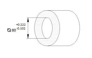
The Problem: A hole has a diameter of 80mm and a tolerance of -0.102 and +0.222. Determine the minimum and maximum dimensions of this hole using Python Jupiter Notebook:)

01_Solution (python cell code):

D=80
a=-0.102
b=0.222
Dmin=D+a
Dmax=D+b
print('Max Diameter: %.3f' % Dmax)
print('Min Diameter: %.3f' % Dmin)

Max Diameter: 80.222 
Min Diameter: 79.898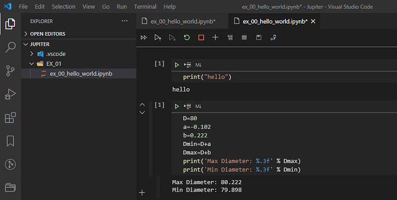

02#PyEx — Python — Compound Rate: In the compound interest modality, the future value is calculated using the formula:

vf = vp * (1 + i) ** n

Where vf is the future value, vp is the present value, i the growth rate and n is the elapsed time;

The Problem: What is the future value of a $ 144,010 investment made in 14 months at a compound interest rate of 1.3% per month?

02_Solution (python cell code):

c=144010.00 
n=14
i=1.3/100
m=c*(1+i)**n
print('The amount is: $ %.2f' %m)

The amount is: $ 172553.94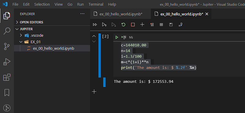

03#PyEx — Python — Roots of a Function:

The Problem: What are the roots of the function: f(x) = -2x³+7x²-20x + 6?

03_Solution (python cell code):

import numpy as np
c=[-2,7,-20,6]
np.roots(c)

array([1.58217509+2.53665299j, 1.58217509–2.53665299j, 0.33564982+0.j ])

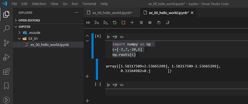
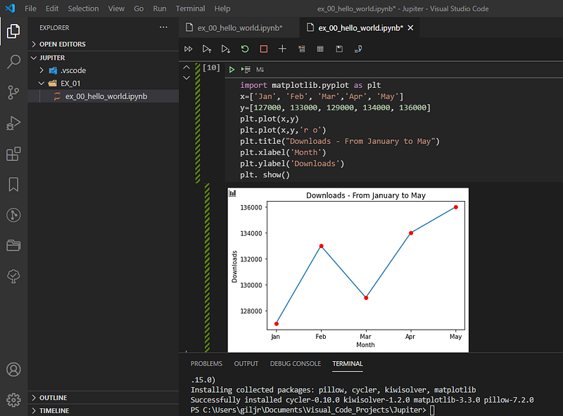
04#PyEx — Python — Tables and Graphs: The following table 1 shows the number of downloads of an application from January to May of the year 2020.

table 1. App Downloads per Month

The Problem: Using python make a graph of lines with circles for each month related to the number of downloads with each of these months;

04_Solution (python cell code):

import matplotlib.pyplot as plt
x=['Jan', 'Feb', 'Mar','Apr', 'May']
y=[127000, 133000, 129000, 134000, 136000]
plt.plot(x,y)
plt.plot(x,y,'r o')
plt.title("Downloads - From January to May")
plt.xlabel('Month')
plt.ylabel('Downloads')
plt. show()

graphic below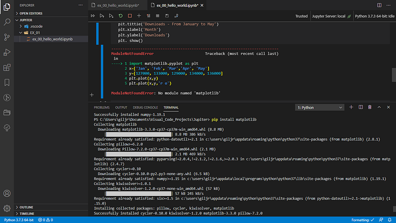

05#PyEx — Python — Pie charts:

The Problem: At McDonald’s international snack chain (the biggest fast-food company in the world), here in Brazil, has sold monthly online over 5226 BigMac, 2404 McSpicy, 3218 Cheeseburger, and 4321 McNuggets;

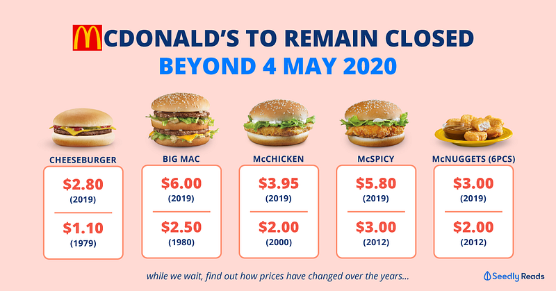
Find Percentage of each product, and show results in a Pie Chart; highlighting the best selling snack of this month; use python, please:)

05_Solution (python cell code):

import matplotlib.pyplot as plt
x=[5226,2404,3218,4321]
snacks=['BigMac','McSpicy','Cheeseburger','McNuggets']
colors=['r','m','y','g']
plt.axis('equal')
plt.pie(x,labels=snacks,colors=colors,shadow=True,explode=  
         (0.1,0,0,0),autopct=('%1.1f%%'))
plt.title('Snacks sold in a month')
plt.show()

graphic below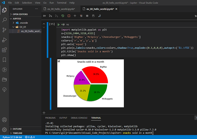

06#PyEx — Python — Derivatives: Derivatives can be used to calculate the profit and loss in business using graphs; to check the temperature variation; to determine the speed or distance covered such as miles per hour, kilometer per hour, to run Lego, Arduino, etc.

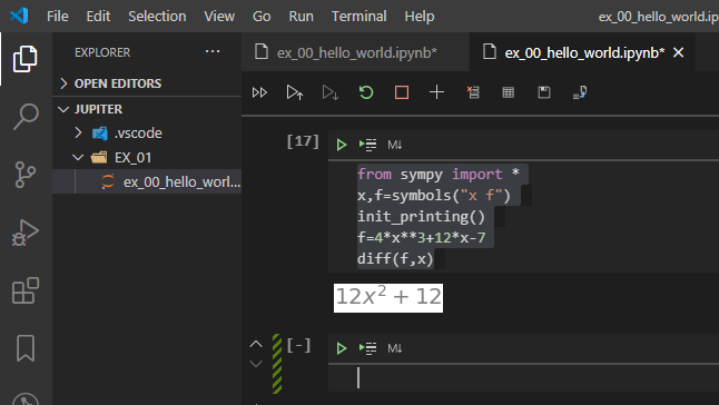
The Problem: Using python, calculate the first derivative of the function: f(x)=4x³+12x-7:

06_Solution (python cell code):

from sympy import *
x,f=symbols("x f")
init_printing()
f=4*x**3+12*x-7
diff(f,x)

12x²+12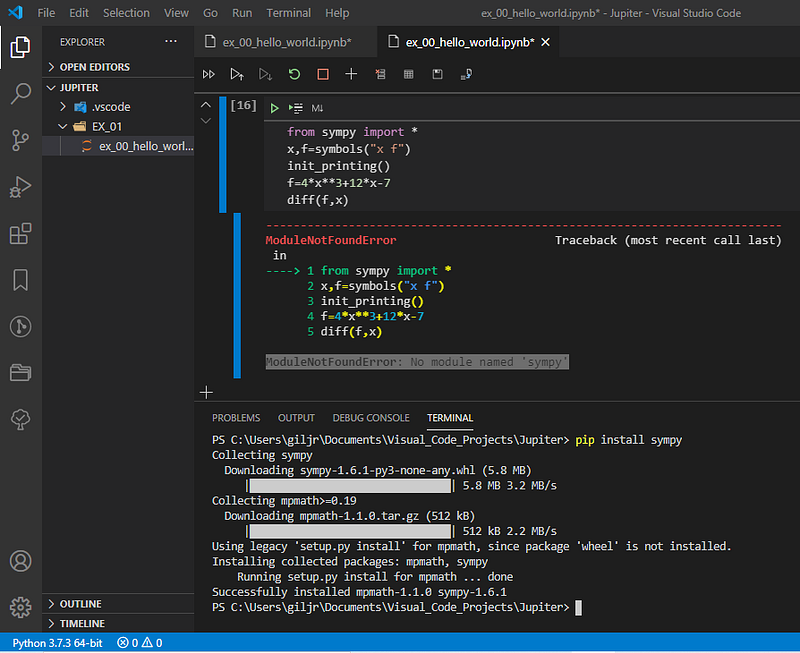

07#PyEx — Python: Indefinite Integral or Antiderivatives — In calculus, an antiderivative, inverse derivative, primitive function, primitive integral, or indefinite integral of a function f is a differentiable function F whose derivative is equal to the original function f. This can be stated symbolically as {\displaystyle F’=f}; The process of solving for antiderivatives is called antidifferentiation (or indefinite integration) and its opposite operation is called differentiation, which is the process of finding a derivative (from https://en.wikipedia.org/wiki/Antiderivative).

The Problem: Calculate the indefinite integral of the function:

f’(x) = 4x³+12x+7;

07_Solution (python cell code):

from sympy import *
x,f=symbols("x f")
init_printing()
f=4*x**3+12*x-7
integrate(f,x)

x⁴+6X²-7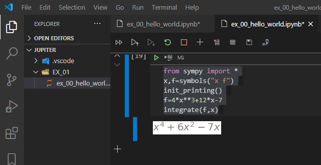

08#PyEx — Python — Linear System:

The Problem: Using python, solve the following linear system:

• 5x+y+3z=76
• -x+2y+5z=35
• 4x-5y+z=22

Edited: April2021 (Python3 adaptation; )

08_Solution (python cell code):

import numpy as np
A = np.array([[5, 1, 3], [-1, 2, 5], [4, -5, 1]])
b = np.array([76, 35, 22])
x = np.linalg.solve(A,b)
print(x)

[10.  5.  7.]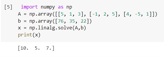

09#PyEx — Python — break-even point (BEP) in Economics:

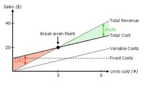
The break-even point (BEP) in economics, business — and specifically cost accounting — is the point at which total cost and total revenue are equal, i.e. “even”. There is no net loss or gain, and one has “broken even”, though opportunity costs have been paid and capital has received the risk-adjusted, expected return. In short, all costs that must be paid are paid, and there is neither profit nor loss:/

The Problem: A company that produces honeycomb polycarbonate has a production cost of $ 129 per unit. Knowing that the sale of the product is $ 193.57 and the monthly production cost is $ 18322.80, obtain, using python, the BEP (I’ll use R for total Revenue, C for total Cost, x for Units sold, xp — x-axis — for the number of products sold to reach BEP point and yp — y-axis — for BEP point in $).

09_Solution (python cell code):

from sympy import *
C,R,x=symbols("C R x")
init_printing()
R=193.57*x
C=129*x+18322.80
xp=solve(Eq(R,C),x)
yp=R.subs(x, xp[0])
print(xp[0])
print(yp)

283.766455010067
54928.6726962986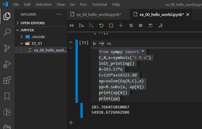

10#PyEx — Python — Linear regression: Linear regression is a common Statistical Data Analysis technique. It is used to determine the extent to which there is a linear relationship between a dependent variable and one or more independent variables. The equation has the form Y= a + bX, where Y is the dependent variable (that’s the variable that goes on the Y-axis), X is the independent variable (i.e. it is plotted on the X-axis), b is the slope of the line and a is the y-intercept.

The Problem: The energy consumption in a residence is shown in table 2 below:

Table 2 — energy consumption

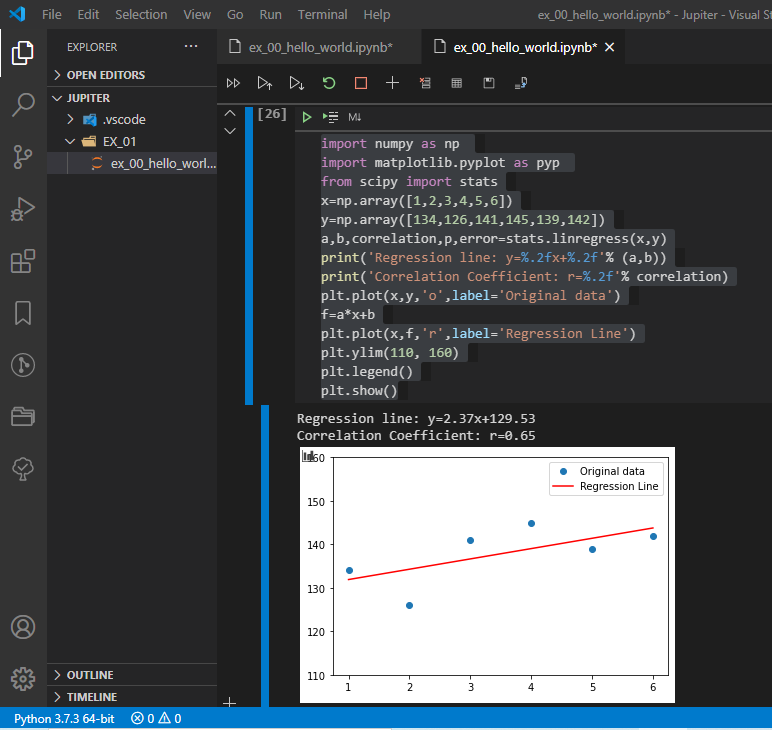
The Problem: Obtain, via python, the regression line, the correlation coefficient, and plot the graph showing the line and the data:

10_Solution (python cell code):

import numpy as np
import matplotlib.pyplot as pyp
from scipy import stats
x=np.array([1,2,3,4,5,6])
y=np.array([134,126,141,145,139,142])
a,b,correlation,p,error=stats.linregress(x,y)
print('Regression line: y=%.2fx+%.2f'% (a,b))
print('Correlation Coefficient: r=%.2f'% correlation)
plt.plot(x,y,'o',label='Original data')
f=a*x+b
plt.plot(x,f,'r',label='Regression Line')
plt.ylim(110, 160)
plt.legend()
plt.show()

Regression line: y=2.37x+129.53 
Correlation Coefficient: r=0.65
graphic below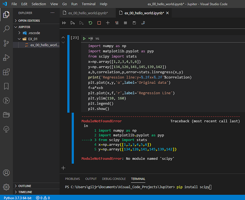

11#PyEx — Python — Parabolic Function: parabolic shape helps ensure that the bridge stays up and that the cables can sustain the weight of hundreds of cars and trucks each hour.

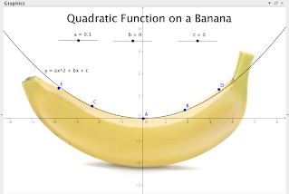
The Problem: Obtain the parabola equation knowing that the points a (0,0), b (10,5), and c (20,0), in meters, belong to the structure of a bridge.

11_Solution (python cell code):

from scipy.interpolate import *
x=[0,10,20]
y=[0,5,0]
f=lagrange(x,y)
print(f)

-0.05x²+x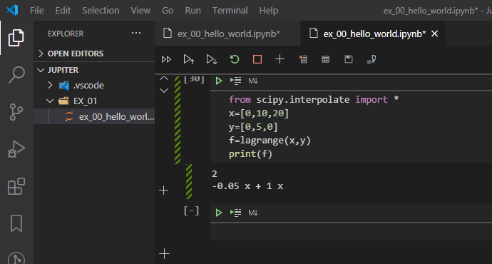

12#PyEx — Python — Linear programming (LP): LP is a tool for solving optimization problems. In 1947, George Dantzig developed an efficient method, the simplex algorithm, for solving linear programming problems (also called LP). Since the development of the simplex algorithm, LP has been used to solve optimization problems in industries as diverse as banking, education, forestry, petroleum, and trucking. In a survey of Fortune 500 firms, 85% of the respondents said they had used linear programming, as a measure of the importance of linear programming in operations research:

Search for LP:

(Introduction to Linear Programming from ufrgs.br).

or

(http://www.optimization-online.org/DB_FILE/2011/09/3178.pdf)

The Problem: A Carrier Corporation has its deliveries optimized.

But on one day, one of his vehicles suffered an unusual attack:) was temporarily inoperative…

Now you need to formulate a Plan B for the delivery of two sets of important products A and B.

Each box of Product A weighs 20 kg and occupies 0.45m³.

Each box of Product B weighs 30 kg and occupies 0.35m³.

The profit for transporting Product A is $ 4.10.

The profit for transporting Product B is $ 5.40.

The truck has the capacity to transport 2 tons and the space of 30m³.

Knowing that the carrier wants to transport as many products as possible and obtain the highest possible profit, use linear programming, and solve the problem.

12_Solution (python cell code):

import sys
!{sys.executable} -m pip install pulp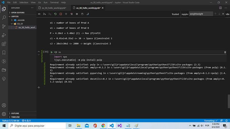

from pulp import *
prob=LpProblem('Example', LpMaximize)
x1=LpVariable("Product A", 0)
x2=LpVariable("Product B", 0)
prob += 4.10*x1 + 5.40*x2
prob += 0.45*x1+0.35*x2 <= 30
prob += 20*x1+30*x2 <= 2000
prob.solve()
for v in prob.variables():
    print(v.name,"=", v.varValue)
print("Max Profit = ", value(prob.objective))

Product_A = 30.769231 
Product_B = 46.153846 
Max Profit =  375.3846155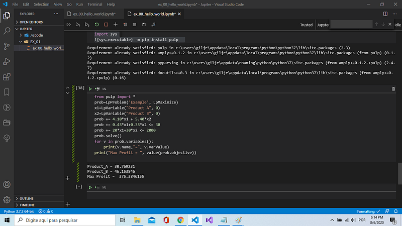

And finally, that’s all!

I hope you can be as surprised just as I am surprised by the 💪Power of Python!

See you in the next PySeries!

Bye, for now, o/

Download all Files from the GitHub Repo

References & Credits

Thank you, Mr. Ricardo A. Deckmann Zanardini — You are an Awesome Teacher! o/; Text edited while I’m studying Computer Engineer at Escola Superior Politécnica Uninter🏋!

Visualizing quaternions (4d numbers) with stereographic projection — from 3Blue1Brown

Introduction to Linear Programming from ufrgs.br (Universidade Federal do Rio Grande do Sul — Brazil)

PuLP: A Linear Programming Toolkit for Python by optimization-online.org

Posts Related:

00Episode#PySeries — Python — Jupiter Notebook Quick Start with VSCode — How to Set your Win10 Environment to use Jupiter Notebook

01Episode#PySeries — Python — Python 4 Engineers — Exercises! An overview of the Opportunities Offered by Python in Engineering! (this one:)

02Episode#PySeries — Python — Geogebra Plus Linear Programming- We’ll Create a Geogebra program to help us with our linear programming

03Episode#PySeries — Python — Python 4 Engineers — More Exercises! — Another Round to Make Sure that Python is Really Amazing!

04Episode#PySeries — Python — Linear Regressions — The Basics — How to Understand Linear Regression Once and For All!

05Episode#PySeries — Python — NumPy Init & Python Review — A Crash Python Review & Initialization at NumPy lib.

06Episode#PySeries — Python — NumPy Arrays & Jupyter Notebook — Arithmetic Operations, Indexing & Slicing, and Conditional Selection w/ np arrays.

07Episode#PySeries — Python — Pandas — Intro & Series — What it is? How to use it?

08Episode#PySeries — Python — Pandas DataFrames — The primary Pandas data structure! It is a dict-like container for Series objects

09Episode#PySeries — Python — Python 4 Engineers — Even More Exercises! — More Practicing Coding Questions in Python!

10Episode#PySeries — Python — Pandas — Hierarchical Index & Cross-section — Open your Colab notebook and here are the follow-up exercises!

11Episode#PySeries — Python — Pandas — Missing Data — Let’s Continue the Python Exercises — Filling & Dropping Missing Data

12Episode#PySeries — Python — Pandas — Group By — Grouping large amounts of data and compute operations on these groups

13Episode#PySeries — Python — Pandas — Merging, Joining & Concatenations — Facilities For Easily Combining Together Series or DataFrame

14Episode#PySeries — Python — Pandas — Pandas Dataframe Examples: Column Operations

15Episode#PySeries — Python — Python 4 Engineers — Keeping It In The Short-Term Memory — Test Yourself! Coding in Python, Again!

16Episode#PySeries — NumPy — NumPy Review, Again;) — Python Review Free Exercises

17Episode#PySeries — Generators in Python — Python Review Free Hints

18Episode#PySeries — Pandas Review…Again;) — Python Review Free Exercise

19Episode#PySeries — MatlibPlot & Seaborn Python Libs — Reviewing theses Plotting & Statistics Packs

20Episode#PySeries — Seaborn Python Review — Reviewing theses Plotting & Statistics Packs