Statistical Techniques for Anomaly Detection (Part 2) Grubb’s Test, Univariate and Multivariate Anomalies

A carefully generated, thoroughly engineered resource for Data Scientists.

Part 2 of Chapter 02 from the Guide to Machine Learning for Anomaly Detection

Warning! Before you continue reading this article and all the articles that compose this guide, you must understand this was in part generated using OpenAI’s GPT 4 model. It started as a self learning project and I soon enough realized this could be really valuable to fellow data scientists. Because of this, I will release the entire guide for free alongside every chapter so you can directly go read the guide from the document so you don’t even need to give me reading time if you don’t want to.

Guide Index

Coding Time: Detecting Outliers with Grubbs’ Test

Grubbs’ Test, also known as the Maximum Normal Residual Test, is a

statistical test that identifies potential outliers in a univariate dataset that follows an approximately normal distribution.

Named after Frank E. Grubbs who developed it in 1950, the test operates under the null hypothesis that there are no outliers in the data.

Grubbs’ Test:

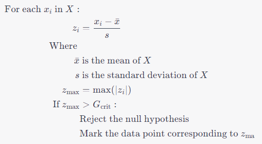
determines the z-score of each data point (the number of standard deviations the point is from the mean), and then
selects the data point with the highest absolute z-score.
If this maximum z-score exceeds the Grubbs’ critical value, then the null hypothesis is rejected, and the corresponding data point is marked as an outlier.

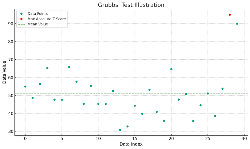
Let’s illustrate this test with a Python code snippet.

import numpy as np
import scipy.stats as stats

# Set the random seed for reproducibility
np.random.seed(0)

# Generate 30 data points from a normal distribution with mean 0 and standard deviation 1
data = np.random.normal(0, 1, 30)

# Introduce an outlier
data[15] = 3.5

# Define Grubbs' Test function
def grubbs_test(data, alpha=0.05):
    n = len(data)
    mean = np.mean(data)
    std_dev = np.std(data)
    z_scores = (data - mean) / std_dev
    abs_z_scores = np.abs((data - mean) / std_dev)
    max_z_score = np.max(abs_z_scores)
    max_z_score_index = np.argmax(abs_z_scores)
    
    print(f"Number of data points: {n}")
    print(f"Mean of data: {mean}")
    print(f"Standard Deviation of data: {std_dev}")
    print("\nZ-Scores")
    print(z_scores)
    print(f"Max Absolute Z-Score: {max_z_score} located at index {max_z_score_index}\n")

    # Calculate the Grubbs' Test statistic
    G_calculated = (n-1) * np.sqrt(max_z_score**2 / (n-2+max_z_score**2))

    # Look up the critical value of the Grubbs' Test statistic from the t-distribution
    t_critical = stats.t.ppf(1 - alpha / (2*n), n-2)
    G_critical = ((n-1) / np.sqrt(n)) * np.sqrt(t_critical**2 / (n-2 + t_critical**2))

    # If the calculated test statistic is larger than the critical value, then reject the null hypothesis and mark the data point as an outlier
    if G_calculated > G_critical:
        print(f"Outlier detected at index {max_z_score_index}.")
        outlier = True
    else:
        print("No outliers detected.")
        outlier = False

    return max_z_score_index, outlier


# Call the Grubbs' Test function on our data
outlier_index, is_outlier = grubbs_test(data)

Number of data points: 30 Mean of data: 0.548400636350699 Standard Deviation of data: 1.2125864203903554

Z-Scores [ 1.00252789 -0.12225391 0.35489211 1.39577067 1.08788729 -1.25820188 0.33126528 -0.57707874 -0.53737983 -0.11364315 -0.3334666 0.7470584 0.1753583 -0.35191357 -0.08621027 2.43413526 0.77988539 -0.62144758 -0.19407519 -1.1566156 -2.5576655 0.08677151 0.26062931 -1.06430819 1.41957221 -1.65164831 -0.41452066 -0.60662438 0.81180076 0.75949897]

Max Absolute Z-Score: 2.557665499162014 located at index 20

Outlier detected at index 20.

# Create a scatter plot of the data
import matplotlib.pyplot as plt

plt.figure(figsize=(10, 6))
plt.scatter(range(len(data)), data, color='blue', label='Data points')
if is_outlier:
    plt.scatter(outlier_index, data[outlier_index], color='red', label='Outlier')
plt.axhline(y=np.mean(data), color='green', linestyle='-', label='Mean')
plt.legend()
plt.title('Data points and Outlier')
plt.xlabel('Index')
plt.ylabel('Value')
plt.show()

# Create a histogram of the data
plt.figure(figsize=(10, 6))
plt.hist(data, bins=20, color='blue', alpha=0.7, label='Data points')
if is_outlier:
    plt.axvline(x=data[outlier_index], color='red', linestyle='-', label='Outlier')
plt.axvline(x=np.mean(data), color='green', linestyle='-', label='Mean')
plt.legend()
plt.title('Histogram and Outlier')
plt.xlabel('Value')
plt.ylabel('Frequency')
plt.show()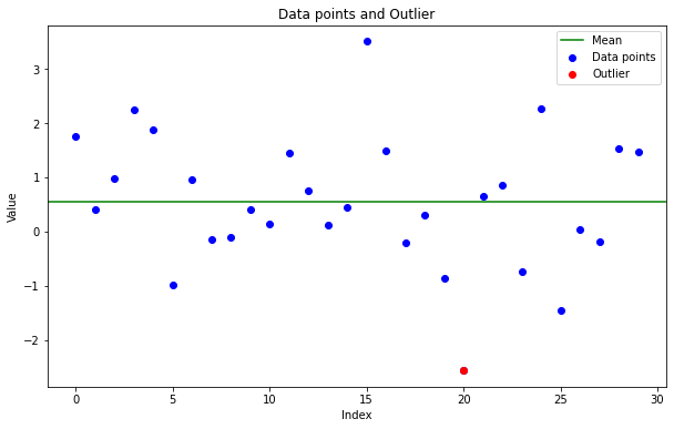

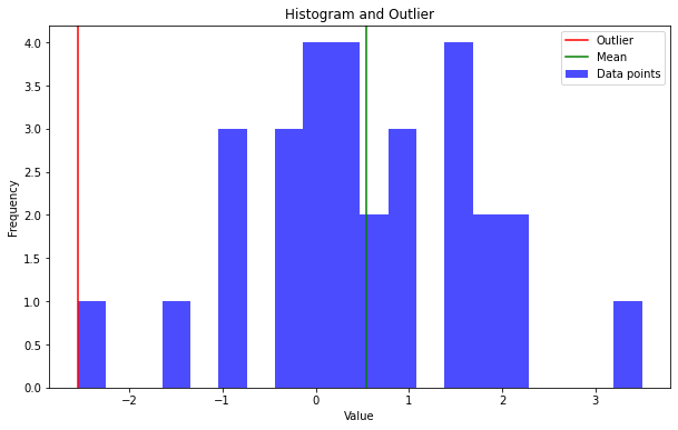
In the code above, we begin by generating 30 data points from a standard normal distribution and introduce an outlier (the 15th data point is set to 3.5). We then define a function for Grubbs’ Test, which

calculates the z-score of each data point, determines the data point with the maximum z-score, and then compares the test statistic of this maximum z-score with the critical value from the Grubbs’ Test.

If the test statistic exceeds the critical value, the function identifies this data point as an outlier.

This example demonstrates how Grubbs’ Test can be an effective tool for detecting outliers in a univariate dataset. However, like all statistical tests, it’s essential to be aware of its assumptions and limitations. In this case, Grubbs’ Test assumes the data is normally distributed and identifies only one outlier at a time. If there are multiple outliers, the test needs to be applied iteratively, removing one outlier at a time and recalculating the test statistic.

Grubbs’ Test is designed to test for a single outlier at a time in normally distributed datasets.

This means that if there is more than one outlier in the dataset, Grubbs’ Test will only identify the most extreme one.

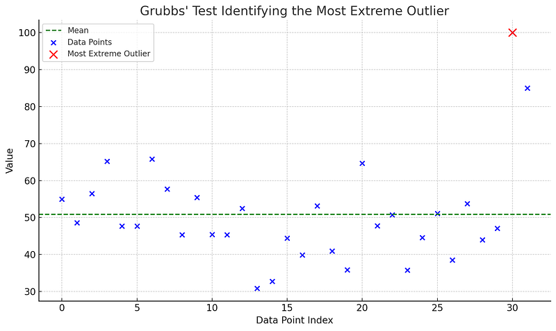
As we can observe, even though there are two outliers in the dataset, Grubbs’ Test has only highlighted the most extreme one. This demonstrates the concept that Grubbs’ Test is designed to test for a single outlier at a time in normally distributed datasets.

If you suspect that there may be multiple outliers in your dataset, you could apply Grubbs’ Test iteratively. In each iteration, you remove the most extreme outlier detected by the test (provided that the test indicates it is indeed an outlier), and then reapply the test to the remaining data. This process can be continued until no further outliers are detected.

However, keep in mind that this iterative procedure may increase the chances of Type I error (false positives), especially if the dataset is large or if the number of true outliers is small. This is because the more tests you perform, the greater the chance that you’ll find an “outlier” just by chance. Therefore, if you’re planning to use Grubbs’ Test iteratively, it’s important to use a suitable method to control the family-wise error rate, such as the Bonferroni correction.

Lastly, note that Grubbs’ Test is sensitive to the assumption of normality. If the dataset does not approximately follow a normal distribution, the results of the test may not be reliable. In such cases, a non-parametric method for outlier detection might be more appropriate.

Univariate and Multivariate Anomalies

When examining data for anomalies or outliers, we often come across two main categories of anomalies — univariate and multivariate. Both types offer valuable insights into the data, but their identification and interpretation require different strategies.

Univariate Anomalies

Univariate anomalies occur within a single feature or variable of the data.

These are instances where the specific data point significantly deviates from the expected pattern or range for that particular variable. This kind of anomalies are the easiest to detect as they involve investigating each variable independently.

For instance, consider a dataset that captures the daily temperature readings for a specific location over the period of one month.

Day | Temperature (°C) 1 | 20.1 2 | 21.2 3 | 20.5 4 | 29.0 5 | 20.8 6 | 21.1 7 | 20.4 … | …

In this dataset, a temperature reading of 29.0°C on the 4th day might be considered as a univariate anomaly if the average temperature for this location is around 20°C and rarely exceeds 22°C.

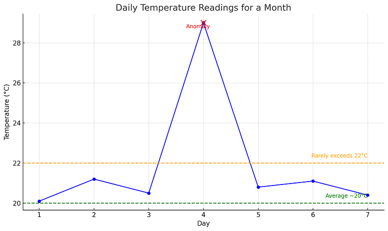
Univariate anomaly detection methods focus on extracting outliers in one dimension or feature at a time. Techniques often used include statistical methods, such as the z-score method or the Grubb’s test, as well as some machine learning-based methods, for example isolation forests or one-class SVM, when the univariate data has a complex distribution.

Multivariate Anomalies

Multivariate anomalies, on the other hand, involve multiple features or variables and occur when a combination of values is considered anomalous, even if the individual values may not be anomalies in their own right.

They are more complex to detect as they involve interactions between multiple variables.

As an example, consider a dataset that captures daily temperature and humidity readings:

Day | Temperature (°C) | Humidity (%) 1 | 20.1 | 50 2 | 21.2 | 51 3 | 20.5 | 52 4 | 20.6 | 95 5 | 20.8 | 50 6 | 21.1 | 49 7 | 20.4 | 52 … | … | …

On the 4th day, the temperature reading of 20.6°C is not an anomaly, and a humidity of 95% might also be usual for some other conditions. However, the combination of 20.6°C and 95% humidity is anomalous for this specific location if it rarely experiences high humidity at moderate temperatures.

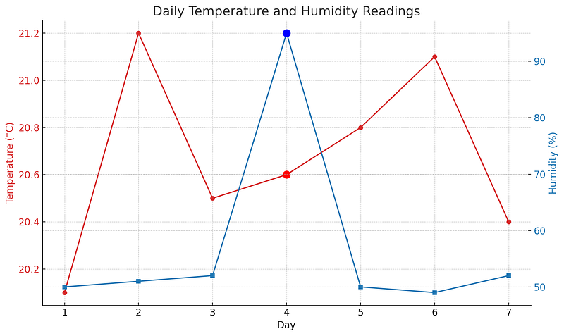
Multivariate anomaly detection methods examine two or more related variables together to identify anomalies. Common techniques for multivariate anomaly detection include

clustering methods (such as k-means or DBSCAN)
classification methods (like SVM or decision trees)
neural networks (like autoencoders)
statistical methods (like the Mahalanobis distance).

Detecting multivariate anomalies can be more beneficial than simply identifying univariate anomalies because real-world systems often involve complex interactions between multiple variables. However, this also means that multivariate anomaly detection can be more computationally intensive and requires a careful choice and tuning of the method used.

In summary, both univariate and multivariate anomalies provide important insights into data. Univariate anomaly detection is a good starting point, but to fully understand complex systems, multivariate anomaly detection is also necessary. The choice of method will depend on the nature of the data and the specific requirements of the analysis.

Coding Time: Detecting Multivariate Outliers with Mahalanobis Distance

When dealing with multivariate data, simple univariate outlier detection methods like Z-score or Grubbs’ test may not be sufficient. Instead, we can use the Mahalanobis Distance, a statistical measure introduced by P. C. Mahalanobis in 1936. It’s effectively a multivariate equivalent of the Z-score.

The Mahalanobis distance considers the covariance between variables, which helps identify patterns that might not be detectable in individual variables.

When data are uncorrelated, Mahalanobis distance equals the Euclidean distance.

Given a data point x in a distribution with mean μ and covariance matrix S, the Mahalanobis distance D is computed as:

D² = (x — μ)’S^(-1)(x — μ)

The square of the Mahalanobis distance follows a Chi-squared distribution, which allows us to perform a hypothesis test to detect outliers.

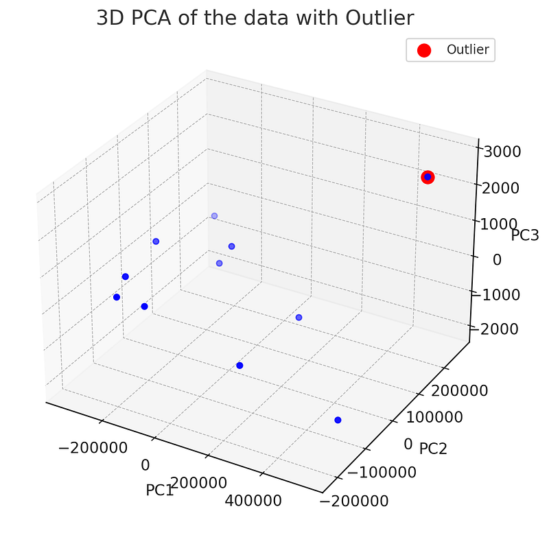
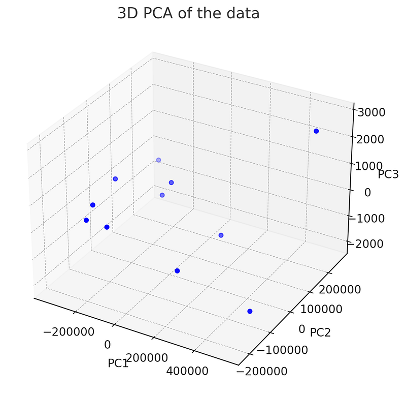
Let’s see this examplee have a small dataset comprising various items or products, each described by multiple attributes such as price, distance, emission, performance, and mileage. By applying the Mahalanobis distance formula, we can calculate the distance between pairs of items in the dataset, which will provide us with a quantitative measure of their dissimilarity or similarity in a multi-dimensional space. This exercise aims to leverage the Mahalanobis distance to identify potential outliers, group similar items, or perform other data analysis tasks to gain valuable insights from the dataset.

Data

| Price | Distance | Emission | Performance | Mileage 0 | 100000 | 16000 | 300 | 60 | 76 1 | 800000 | 60000 | 400 | 88 | 89 2 | 650000 | 300000 | 1230 | 90 | 89 3 | 700000 | 10000 | 300 | 87 | 57 4 | 860000 | 252000 | 400 | 83 | 79 5 | 730000 | 350000 | 104 | 81 | 84 6 | 400000 | 260000 | 632 | 72 | 78 7 | 20 | 260000 | 6302 | 2 | 2000 <<<<<<< 8 | 870000 | 510000 | 221 | 91 | 99 9 | 780000 | 2000 | 142 | 90 | 97 10 | 400000 | 5000 | 267 | 93 | 99

import numpy as np
import pandas as pd
from scipy.stats import chi2
from sklearn.covariance import EmpiricalCovariance

def calculateMahalanobis(data):
    robust_cov = EmpiricalCovariance().fit(data)
    m_dist = robust_cov.mahalanobis(data)
    return m_dist

# Define multivariate data
data = np.array([[100000, 16000, 300, 60, 76],
                 [800000, 60000, 400, 88, 89],
                 [650000, 300000, 1230, 90, 89],
                 [700000, 10000, 300, 87, 57],
                 [860000, 252000, 400, 83, 79],
                 [730000, 350000, 104, 81, 84],
                 [400000, 260000, 632, 72, 78],
                 [20, 260000, 6302, 2, 2000],
                 [870000, 510000, 221, 91, 99],
                 [780000, 2000, 142, 90, 97],
                 [400000, 5000, 267, 93, 99]])

# Create a DataFrame
columns = ['Price', 'Distance', 'Emission', 'Performance', 'Mileage']
df = pd.DataFrame(data, columns=columns)

print(f"Data:\n{df}\n")

# Calculate Mahalanobis distances
m_dist = calculateMahalanobis(df)

print(f"Mahalanobis distances:\n{m_dist}\n")

# Define significance level for outlier detection
alpha = 0.10

# Calculate threshold (based on chi-squared distribution)
thresh = chi2.ppf(1 - alpha, df=df.shape[1])

print(f"Threshold for outlier detection: {thresh}\n")

# Detect outliers (where Mahalanobis distance exceeds threshold)
outliers = df[m_dist > thresh]
df['distance'] = m_dist
df['outlier'] = df['distance'] > thresh

print(f"Outliers:\n{outliers}")

print(f"Data:\n{df}\n")

Mahalanobis distances: [7.23782241 2.22109829 8.21440824 1.89413229 2.57169465 2.83641857 2.70941648 9.99763797 6.10733273 3.03153561 8.17850277]

Threshold for outlier detection: 9.236356899781123

Outliers: | Price | Distance | Emission | Performance | Mileage 7 | 20 | 260000 | 6302 | 2 | 2000

We can review our dataset with the added distance and outlier columns

Data

Price | Distance | Emission | Performance | Mileage | distance | outlier 0 | 100000 | 16000 | 300 | 60 | 76 | 7.237822 | False 1 | 800000 | 60000 | 400 | 88 | 89 | 2.221098 | False 2 | 650000 | 300000 | 1230 | 90 | 89 | 8.214408 | False 3 | 700000 | 10000 | 300 | 87 | 57 | 1.894132 | False 4 | 860000 | 252000 | 400 | 83 | 79 | 2.571695 | False 5 | 730000 | 350000 | 104 | 81 | 84 | 2.836419 | False 6 | 400000 | 260000 | 632 | 72 | 78 | 2.709416 | False 7 | 20 | 260000 | 6302 | 2 | 2000 | 9.997638 | True <<<<<<<<<<< 8 | 870000 | 510000 | 221 | 91 | 99 | 6.107333 | False 9 | 780000 | 2000 | 142 | 90 | 97 | 3.031536 | False 10 | 400000 | 5000 | 267 | 93 | 99 | 8.178503 | False

We can interpret the results as follows:

Mahalanobis Distances: The Mahalanobis distance measures the distance between each data point and the center of the dataset, taking into account the covariance structure of the variables. In this case, we have computed the Mahalanobis distances for each data point in the DataFrame.
Threshold for Outlier Detection: A threshold is established to identify outliers based on the Mahalanobis distance. In this case, the threshold for outlier detection is determined using a significance level of 0.10 (alpha = 0.10) and the number of variables in the dataset. The calculated threshold is 9.236356899781123.
Outliers: Comparing the Mahalanobis distances to the threshold, we can identify the outliers in the dataset. In this case, there is one outlier detected: Data point 7: [20, 260000, 6302, 2, 2000]

This outlier has values that deviate significantly from the rest of the data points, considering the covariance structure of the variables. It exhibits extreme values in multiple dimensions (Price, Distance, Emission, Performance, and Mileage).

See you in chapter 3!

Link to Chapter 2 code : https://github.com/gabrielpierobon/anomaly_detection/blob/main/Chapter%2002%20Statistical%20Techniques%20for%20Anomaly%20Detection.ipynb

Link to PDF Guide: https://drive.google.com/file/d/1g77lB2zeZGQUqIyPSb9Fr-uMyjmAG4j4/view?usp=drive_link