One-Class SVM (Support Vector Machine) for Anomaly Detection
A carefully generated, thoroughly engineered resource for Data Scientists.
Chapter 08 from the Guide to Machine Learning for Anomaly Detection
Warning! Before you continue reading this article and all the articles that compose this guide, you must understand this was in part generated using OpenAI’s GPT 4 model. It started as a self learning project and I soon enough realized this could be really valuable to fellow data scientists. Because of this, I will release the entire guide for free alongside every chapter so you can directly go read the guide from the document so you don’t even need to give me reading time if you don’t want to.

Guide Index
0: About the generation of this guide 1: Introduction to Anomaly Detection 2: Statistical Techniques for Anomaly Detection (Part 1) 2: Statistical Techniques for Anomaly Detection (Part 2) 3: Introduction to M. Learning for Anomaly Detection (Part 1) 3: Introduction to M. Learning for Anomaly Detection (Part 2) 4: Dealing with Imbalanced Classes in Supervised Learning 5: K-Means Clustering for Anomaly detection 6: DBSCAN for Anomaly detection Isolation Forest for Anomaly Detection >>>>> 8: One-Class SVM for Anomaly Detection <<<<< 9: K-Nearest Neighbors (KNN) for Anomaly Detection 10: Principal Graph and Structure Learning (PGSL) for Anomaly Detection 11: Dimensionality Reduction Techniques for Anomaly Detection 12: Singular Value Decomposition (SVD) for Anomaly Detection 13: Advanced Matrix Factorization Techniques for Anomaly Detection 14: Nystrom Method for Anomaly Detection 15: Kernel Methods for Anomaly Detection 16: Advanced Algorithms for Anomaly Detection 17: Feature Selection and Engineering for Anomaly Detection 18: Semi-Supervised Learning for Anomaly Detection 19: Deep Learning for Anomaly Detection 20: Ensemble Methods for Anomaly Detection 21: Evaluation Metrics for Anomaly Detection 22: Case Studies and Industry Applications 23: Conclusion and Future Directions in Anomaly Detection
As we continue our exploration of different methods for anomaly detection, we now turn our attention to a well-known machine learning model, the Support Vector Machine (SVM). However, instead of the conventional binary or multiclass SVM that you may be familiar with,
we will be focusing on a variant of SVM known as One-Class SVM.
One-Class SVM is a unique tool within the SVM family. Rather than identifying the hyperplane (or “decision boundary”) that separates different classes, as is done in conventional SVM,
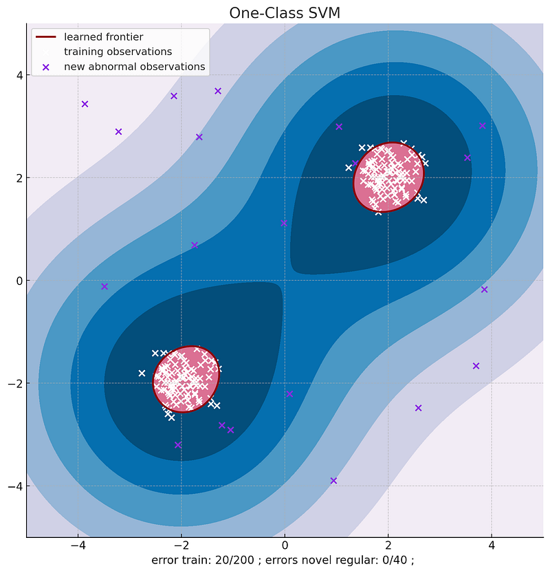
One-Class SVM instead attempts to find the smallest possible hypersphere that encompasses all of the data.
The concept might sound abstract, but the goal here is to capture the “shape” of the data. In doing so, One-Class SVM is capable of identifying novel, anomalous observations that do not conform to this shape.
While One-Class SVM is somewhat less common in practice than other anomaly detection methods we’ve discussed, like K-Means clustering or the Isolation Forest algorithm, it offers a unique perspective on the problem.
Because it seeks to “encapsulate” the normal data, it can sometimes identify anomalies that other algorithms miss.
However, this power comes with a cost.
One-Class SVM can be sensitive to the choice of parameters and it does not scale well to large, high-dimensional datasets.
Despite these drawbacks, it is a valuable addition to your anomaly detection toolbox, offering a robust and nuanced approach to the problem.
In this chapter, we will start by developing an intuition for the One-Class SVM, exploring the underlying theory and how it works. We will then proceed to demonstrate its application using real-world examples. Our goal is to ensure you are equipped with a practical understanding of this method and can implement it to detect anomalies in your own datasets.
As with previous methods, it is crucial to remember that no single algorithm is the “best” solution for every task. Each algorithm has its strengths and weaknesses, and the choice of algorithm should be informed by the specifics of the task, the nature of the data, and the trade-offs you are willing to make. With that in mind, let’s dive into the world of One-Class SVM for anomaly detection.
The Intuition Behind One-Class SVM
Imagine you’re an event security guard tasked with monitoring a gathering and making sure that only invited guests can enter.

If the event is small and the guest list is short, you could possibly remember each of the invitees’ faces. But for a larger event with hundreds or thousands of guests, this would be impossible.
A feasible strategy might be to understand the “characteristics” of the invited guests. Perhaps the event is a tech conference and the guests are mostly IT professionals.
Or maybe it’s a high school reunion and the guests are all roughly the same age. Understanding these patterns could help you spot individuals who seem out of place, even if you don’t know the exact identity of each guest.
One-Class SVM works on a similar principle. Instead of trying to identify each individual data point (or guest), it focuses on understanding the overall pattern or distribution of the data (the crowd of guests). It does this by fitting a boundary around the most dense part of the data, essentially encapsulating the “normal” data points. Then, any observations that lie outside this boundary are considered anomalies.
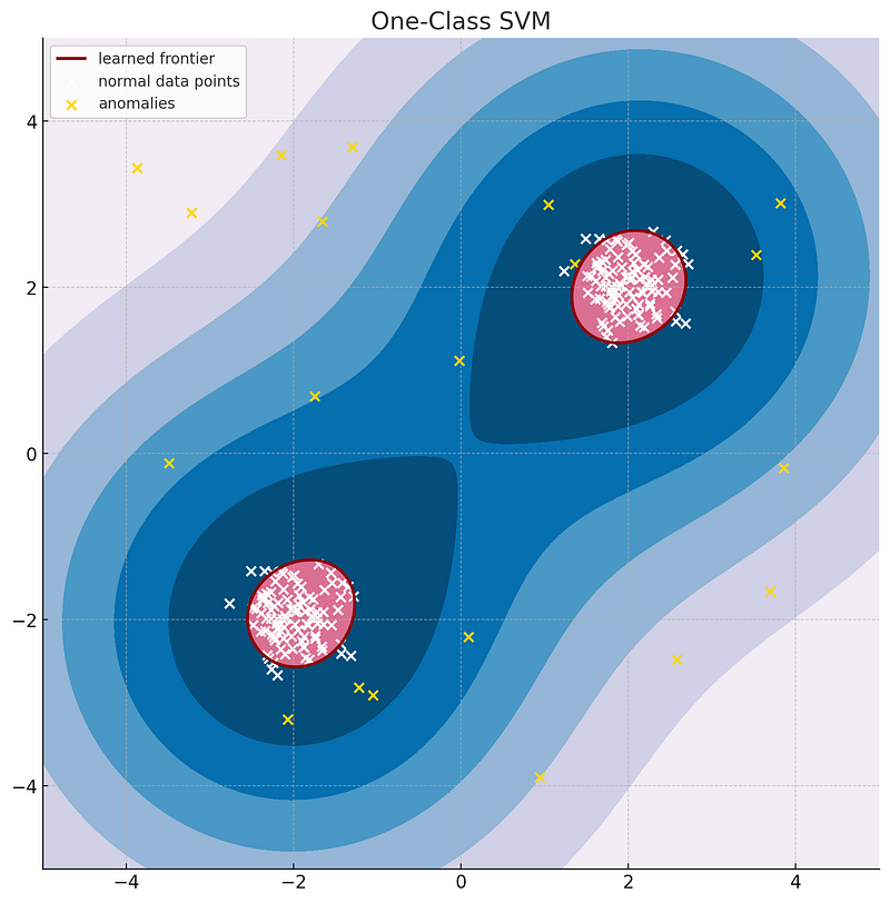
One important point to note is that One-Class SVM is an unsupervised method, meaning it doesn’t require labeled data to identify the boundary. It simply looks for patterns in the data itself. However, the shape and position of this boundary is heavily influenced by the choice of kernel function and the hyperparameters of the algorithm, such as `nu` and `gamma`.
The Theory Behind One-Class SVM
One-Class SVM operates on the principle of finding the smallest hyper-sphere in the feature space that contains all (or most of) the data points.
- Here, “smallest” refers to the idea of creating a boundary that fits closely around the data, rather than being too loose or too tight.
- In the mathematical formulation of One-Class SVM, the origin of the feature space is moved and rescaled so that it coincides with the center of the hyper-sphere and the hyper-sphere has radius 1. The algorithm then tries to maximize the distance from the origin to the hyper-plane (the decision function) subject to some constraints.
- The constraint parameter `nu` controls the trade-off between maximizing the distance from the origin and ensuring that most data points lie inside the hyper-sphere. A larger `nu` value will lead to a smaller hyper-sphere, capturing less of the data, and thus potentially more anomalies.
- The `gamma` parameter, used when the Radial Basis Function (RBF) kernel is chosen, defines the influence of individual training samples — lower values meaning ‘far’ and higher values meaning ‘close’.
- After fitting the One-Class SVM, the decision function provides a score indicating how anomalous each data point is. More negative scores correspond to more anomalous data points.
In the next section, we will walk through the application of One-Class SVM using Python and Scikit-Learn. This practical demonstration will help reinforce these theoretical concepts.
Coding Time: One-Class SVM for Synthetic Data
In this section, we will illustrate how One-Class SVM works using a simple synthetic dataset. A synthetic dataset allows us to visually comprehend the working principle of the algorithm and observe how well it separates normal observations from the outliers.
Creating the Synthetic Dataset: We’ll create a dataset consisting of normally distributed data points and a few outliers.
import numpy as np
from sklearn.svm import OneClassSVM
import matplotlib.pyplot as plt

# Seed for reproducibility
np.random.seed(1)

# Generate training data
X = 0.3 * np.random.randn(100, 2)
X_train = np.r_[X + 2, X - 2]

# Generate some regular novel observations
X = 0.3 * np.random.randn(20, 2)
X_test = np.r_[X + 2, X - 2]

# Generate some abnormal novel observations
X_outliers = np.random.uniform(low=-4, high=4, size=(20, 2))
# Plotting the dataset
plt.scatter(X_train[:, 0], X_train[:, 1], c='white', s=20, edgecolor='k')
plt.scatter(X_test[:, 0], X_test[:, 1], c='blue', s=20, edgecolor='k')
plt.scatter(X_outliers[:, 0], X_outliers[:, 1], c='red', s=20, edgecolor='k')
plt.title("Synthetic Dataset")
plt.show()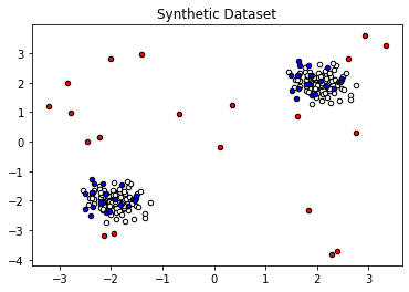
# Fit the model
model = OneClassSVM(nu=0.1, kernel="rbf", gamma=0.1)
model.fit(X_train)
Anomaly Detection: We predict the labels (-1 for an anomaly, 1 for normal) for the test data and the outliers.
y_pred_train = model.predict(X_train)
y_pred_test = model.predict(X_test)
y_pred_outliers = model.predict(X_outliers)
Visualizing the Results: Now, let’s visualize the results by plotting the decision function’s boundary and the anomalies detected by the model.
# Create a meshgrid for the plot
xx, yy = np.meshgrid(np.linspace(-5, 5, 50), np.linspace(-5, 5, 50))
Z = model.decision_function(np.c_[xx.ravel(), yy.ravel()])
Z = Z.reshape(xx.shape)

plt.figure(figsize=(10, 10))
plt.contourf(xx, yy, Z, levels=np.linspace(Z.min(), 0, 7), cmap=plt.cm.PuBu)
a = plt.contour(xx, yy, Z, levels=[0], linewidths=2, colors='darkred')
plt.contourf(xx, yy, Z, levels=[0, Z.max()], colors='palevioletred')

s = 40
b1 = plt.scatter(X_train[:, 0], X_train[:, 1], c='white', s=s, edgecolors='k')
b2 = plt.scatter(X_test[:, 0], X_test[:, 1], c='blue', s=s, edgecolors='k')
c = plt.scatter(X_outliers[:, 0], X_outliers[:, 1], c='red', s=s, edgecolors='k')
plt.axis('tight')
plt.xlim((-5, 5))
plt.ylim((-5, 5))
plt.legend([a.collections[0], b1, b2, c],
           ["Learned frontier", "Training observations",
            "New regular observations", "New abnormal observations"],
           loc="upper left",
           prop=matplotlib.font_manager.FontProperties(size=11))
plt.xlabel("Error train: %d/%d ; errors novel regular: %d/%d ; "
           "errors novel abnormal: %d/%d"
           % (y_pred_train[y_pred_train == -1].size, y_pred_train.size,
              y_pred_test[y_pred_test == -1].size, y_pred_test.size,
              y_pred_outliers[y_pred_outliers == 1].size, y_pred_outliers.size))
plt.show()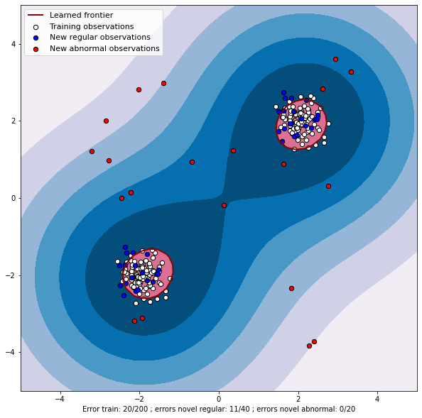
In this example, we have used the synthetic dataset to illustrate how the One-Class SVM model identifies and separates normal data points from anomalies. The model learns a soft boundary in order to isolate the normal data points and uses this boundary to classify new points as similar (normal) or different (anomalies). As you can see, the model has done a good job at detecting the anomalous points in the synthetic dataset.
Coding Time: One-Class SVM for Credit Card Fraud Detection
We are now going to use the One-Class SVM model to detect anomalies in our creditcard.csv dataset.
# Import the necessary libraries
from sklearn import svm
from sklearn.preprocessing import StandardScaler
from sklearn.decomposition import PCA
from sklearn.metrics import confusion_matrix

# Load the dataset
data = pd.read_csv('creditcard.csv')

# Set the fraction of data to sample
fraction = 0.25

# We will use stratified sampling to maintain the ratio of anomalies
stratified_data = data.groupby('Class', group_keys=False).apply(lambda x: x.sample(frac=fraction))

# Separate out the features and labels
X_sample = stratified_data.drop('Class', axis=1)
y_sample = stratified_data['Class']

# Standardize the features to have a mean of ~0 and a variance of 1
scaler = StandardScaler()
X_std_sample = scaler.fit_transform(X_sample)

# Apply PCA to reduce dimensions
pca = PCA(n_components=2)
X_pca_sample = pca.fit_transform(X_std_sample)

# Fit the model only on the normal transactions
model = svm.OneClassSVM(nu=0.1, kernel="rbf", gamma=0.01)
model.fit(X_pca_sample[y_sample == 0])

# Predict the labels for the entire dataset
y_pred_sample = model.predict(X_pca_sample)

# Convert the prediction values to match with 'Class' column in the original dataset
y_pred_sample[y_pred_sample == 1] = 0
y_pred_sample[y_pred_sample == -1] = 1

# Print the confusion matrix
print(confusion_matrix(y_sample, y_pred_sample))
[[63970 7109] [ 62 61]]
This confusion matrix represents the performance of the model. Here is what each part of the matrix represents:
- The top left value (63970) is the number of True Negatives. This means the number of “Normal” (Class 0) transactions that were correctly identified by the model as “Normal”.
- The top right value (7109) is the number of False Positives. This means the number of “Normal” transactions that were wrongly identified by the model as “Fraud” (Class 1).
- The bottom left value (62) is the number of False Negatives. This means the number of “Fraud” transactions that were wrongly identified by the model as “Normal”.
- The bottom right value (61) is the number of True Positives. This means the number of “Fraud” transactions that were correctly identified by the model as “Fraud”.
So, in summary, our model has correctly identified a majority of the “Normal” transactions, but it has also misclassified a significant number of them as “Fraud”. On the other hand, the model has correctly identified a small portion of “Fraud” transactions, but it has missed a roughly equal number of them.
Given the high number of False Positives, the model seems to be overly cautious, flagging many normal transactions as potentially fraudulent. It may require additional tuning to reduce this number and improve the precision of the model. However, the relatively low number of False Negatives indicates that the model is doing well at catching most of the actual fraudulent transactions, which is a good sign. The balance between these two types of errors will depend on the specific cost associated with each in a real-world context.
Finally let’s plot a 2d representation of the dataset and our SVM Classifier:
import matplotlib.pyplot as plt
import matplotlib
import numpy as np

# Generate a grid for the plot
xx, yy = np.meshgrid(np.linspace(-5, 5, 500), np.linspace(-5, 5, 500))

# Predict the scores over the grid
Z = model.decision_function(np.c_[xx.ravel(), yy.ravel()])

# Reshape the scores to the grid
Z = Z.reshape(xx.shape)

plt.figure(figsize=(10, 10))

# Plot the decision boundary
plt.contourf(xx, yy, Z, levels=np.linspace(Z.min(), 0, 7), cmap=plt.cm.PuBu)
a = plt.contour(xx, yy, Z, levels=[0], linewidths=2, colors='darkred')

# Plot data points
b1 = plt.scatter(X_pca_sample[y_sample==0, 0], X_pca_sample[y_sample==0, 1], c='white', s=20, edgecolors='k')
b2 = plt.scatter(X_pca_sample[y_sample==1, 0], X_pca_sample[y_sample==1, 1], c='blue', s=20, edgecolors='k')

plt.axis('tight')
plt.xlim((-5, 5))
plt.ylim((-5, 5))

plt.legend([a.collections[0], b1, b2],
           ["learned frontier", "normal transactions", "fraud transactions"],
           loc="upper left",
           prop=matplotlib.font_manager.FontProperties(size=11))

plt.title("One-Class SVM")
plt.xlabel("Principal Component 1")
plt.ylabel("Principal Component 2")

plt.show()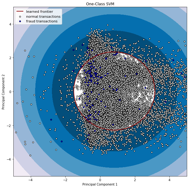
In this chapter, we delved into the depths of One-Class SVM, a novel approach for tackling the challenge of anomaly detection. We explored the concept and intuition behind this machine learning algorithm, its theoretical underpinnings, and how it can be implemented using Python. We demonstrated its power using a synthetic dataset and then on a real-world financial dataset, showcasing its capacity to identify outliers in a multi-dimensional space.
We observed the trade-offs in using One-Class SVM, particularly in balancing false positives and negatives, and discussed the relevance of fine-tuning the model to suit specific use-cases. We also addressed the computational intensity of the algorithm, particularly when dealing with high-dimensional, large-scale datasets. This necessitated sampling strategies, like the one we used with the credit card dataset, to ensure that the model was computationally feasible.
We visualized the decision boundary created by the One-Class SVM and illustrated how it efficiently encapsulates the normal data and separates it from the anomalies. These visualizations were crucial in enhancing our understanding of the One-Class SVM’s working mechanism, as well as its strengths and limitations.
Our experiment with One-Class SVM highlights its utility as a powerful tool for anomaly detection, suitable for applications where the positive (normal) class is well-defined, while the negative class (anomalies) is vaguely characterized or not well-sampled. However, it also emphasizes the importance of proper parameter tuning, feature engineering, and post-model analysis, like checking the feature importance and providing model explainability.
See you in Chapter 9!


