Introduction to Machine Learning for Anomaly Detection (Part 1)

A carefully generated, thoroughly engineered resource for Data Scientists.

Part 1 of Chapter 03 from the Guide to Machine Learning for Anomaly Detection

Warning! Before you continue reading this article and all the articles that compose this guide, you must understand this was in part generated using OpenAI’s GPT 4 model. It started as a self learning project and I soon enough realized this could be really valuable to fellow data scientists. Because of this, I will release the entire guide for free alongside every chapter so you can directly go read the guide from the document so you don’t even need to give me reading time if you don’t want to.

Guide Index

In the world of data, anomalies are like a needle in the haystack. They are rare, different, and hidden among vast amounts of normal data. However, these anomalies often hold the most valuable information. Spotting credit card fraud, detecting system faults in real-time, identifying rare diseases in healthcare, and many such critical tasks heavily depend on our ability to detect these anomalies accurately and efficiently.

In previous chapters, we explored statistical methods to detect anomalies in both univariate and multivariate datasets. These methods, like Z-Score, Grubbs’ Test, Chi-Square Test, and Mahalanobis Distance, provided us with valuable tools to deal with simple scenarios and specific types of data distributions. However, real-world datasets often come with a higher level of complexity, featuring attributes such as non-linear patterns, high-dimensionality, noise, and intricate dependencies among variables. In these circumstances, traditional statistical methods may falter, struggling to capture the nuanced patterns that separate anomalies from normal data points.

To address the limitations of statistical methods and to provide a more robust and sophisticated approach to anomaly detection, we turn to Machine Learning (ML).

Machine Learning, a subset of Artificial Intelligence (AI), focuses on developing algorithms that can learn from and make decisions based on data. It can uncover hidden patterns, identify correlations, and predict future outcomes based on historical data, making it an effective tool for anomaly detection.

Machine Learning for anomaly detection is akin to training a digital detective. This detective observes, learns from the data, understands what constitutes normal behavior, and then applies this knowledge to detect instances that deviate from the norm.

Unlike humans, ML algorithms can sift through vast amounts of data tirelessly, scaling the anomaly detection process to handle large-scale datasets encountered in real-world applications.

Machine Learning models for anomaly detection can handle the complexity and the diversity of real-world data. They can identify anomalies in high-dimensional data spaces, capture complex non-linear relationships between variables, and adapt to changing data patterns over time. With the power of ML, we can detect anomalies in a variety of contexts, from detecting fraudulent transactions in real-time financial data, spotting intrusions in network traffic, identifying system faults in manufacturing processes, to finding abnormal patterns in healthcare data.

In this chapter, we will explore how Machine Learning comes to our aid in the quest for anomaly detection. We will dive into the types of ML-based anomaly detection techniques, understand their working principles, and implement them using Python.

Supervised vs Unsupervised Learning

Before delving into the specifics of Machine Learning (ML) techniques for anomaly detection, it is vital to understand the different learning paradigms that these techniques fall into.

In the realm of ML, the two fundamental paradigms are Supervised Learning and Unsupervised Learning.

Each paradigm has its characteristics, use cases, advantages, and limitations. This section aims to draw a clear distinction between these two paradigms and to shed light on their role in anomaly detection.

Supervised Learning

In Supervised Learning, the learning process is guided by a teacher — hence the term ‘supervised’. The teacher, in this case, is a pre-existing set of examples (the training data), where the correct output (the label) is known for each input.

The primary task in Supervised Learning is to learn a mapping from inputs to outputs, or in other words, to predict the output label given the input data. This is achieved by training a model on the labeled training data, and then this trained model can make predictions on unseen data.

Supervised Learning can further be categorized into two types:

Classification
Regression.

In classification, the output is a category (e.g., ‘fraudulent’ or ‘non-fraudulent’ transaction), whereas, in regression, the output is a continuous value (e.g., the price of a house).

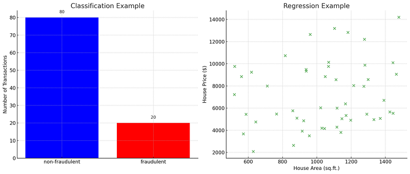
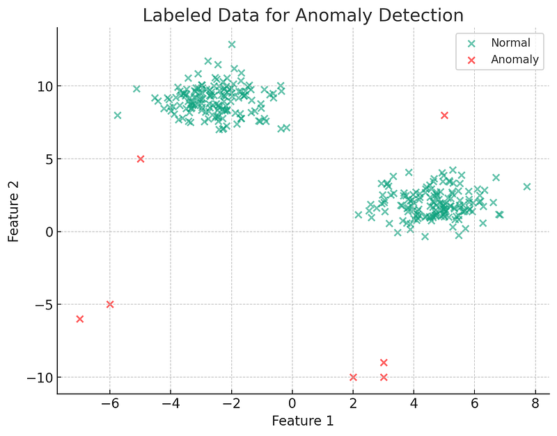
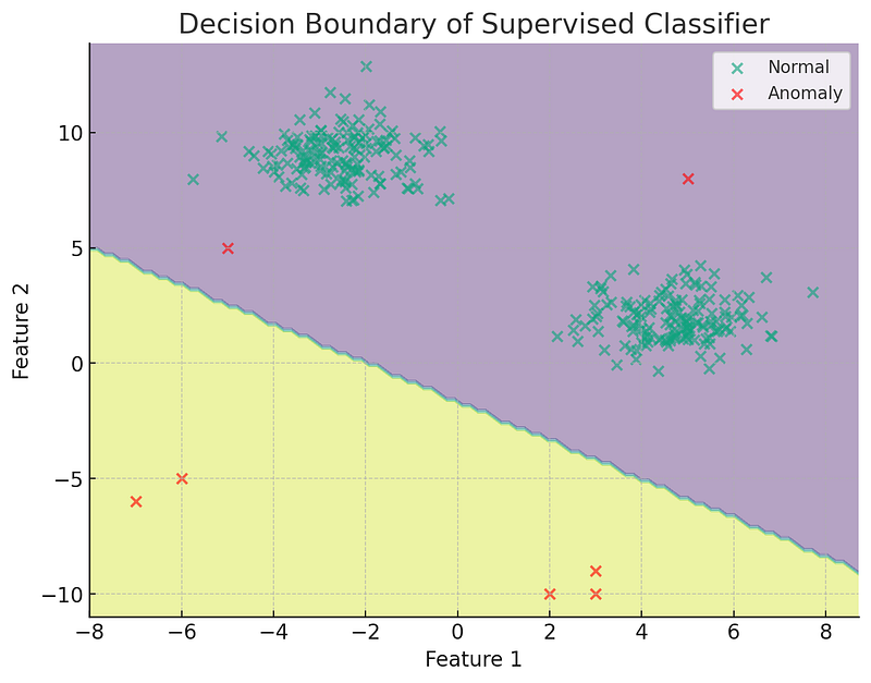
In the context of anomaly detection, Supervised Learning can be highly effective when we have labeled data, i.e., when we know which data points are anomalies and which are not. The ML model can learn the characteristics of normal and anomalous examples during training, and then it can accurately classify new data points as normal or anomalous. However, obtaining labeled data for anomaly detection is challenging as anomalies are rare and often unknown in advance.

Unsupervised Learning

Unlike Supervised Learning, Unsupervised Learning does not rely on labeled training data. Instead, it tries to learn the underlying structure or distribution of the data in order to make inferences about new, unseen data. Unsupervised Learning algorithms can discover interesting patterns in the data, group similar data together (clustering), reduce dimensionality, and more.

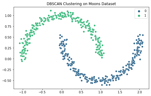
Unsupervised Learning is particularly relevant for anomaly detection for several reasons.

First, anomalies are typically rare events, and in many cases, we do not have any labeled anomalies in the training data. Unsupervised Learning methods can deal with this situation by learning the normal data’s structure and then identifying data points that deviate from this normal structure as anomalies.
Second, the nature of anomalies can change over time (a phenomenon known as concept drift), making it hard to rely on past anomaly labels. Unsupervised methods, which focus on the structure of the normal data, can adapt to these changes.

In conclusion, both Supervised and Unsupervised Learning have their place in the toolbox of anomaly detection. The choice between them depends largely on the availability of labeled data and the specific nature of the anomaly detection problem at hand. In the following sections, we will explore specific ML techniques for anomaly detection under these two paradigms.

Semi-Supervised Learning

Imagine a scenario where you have a large dataset, but only a tiny fraction of it is labeled. Labeling data can be expensive, time-consuming, and requires domain expertise, which might not be readily available. In such cases, Semi-Supervised Learning comes into play.

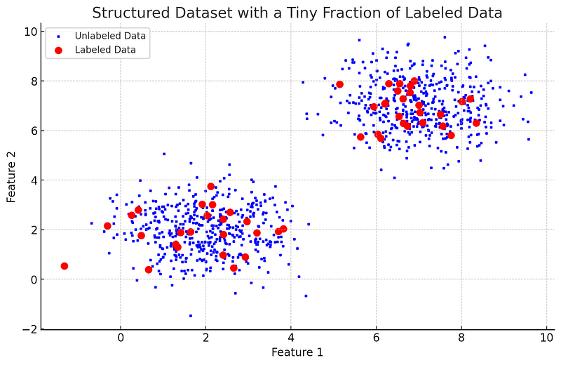
This learning paradigm leverages the power of Unsupervised Learning to understand the underlying structure of the data and the patterns that exist within. Simultaneously, it uses the available labeled data to guide its learning process, making predictions or classifications much like Supervised Learning.

The intuition behind this approach is that the data distribution can help build an effective model, and the limited labeled data can guide this model in the right direction.

By leveraging both labeled and unlabeled data, Semi-Supervised Learning can often achieve higher accuracy than purely Supervised or Unsupervised methods, especially when the amount of labeled data is scarce.

Semi-Supervised Learning in Anomaly Detection

In the context of anomaly detection, Semi-Supervised Learning can be particularly useful. As mentioned earlier, anomalies are rare events that occur infrequently. Therefore, in many real-world scenarios, we have a large amount of normal (non-anomalous) data and a very small amount of anomalous data.

Under such conditions, Semi-Supervised Learning techniques can shine:

The model is initially trained on the normal data (unlabeled) to understand what normal behavior looks like.
The limited anomalous instances (labeled data) are then used to fine-tune the model’s understanding of what constitutes an anomaly.
Consequently, the model becomes proficient at differentiating between normal and anomalous instances.

Introduction to Algorithms for Anomaly Detection

Supervised Learning Algorithms for Anomaly Detection

Supervised learning algorithms require labeled data for training, i.e., we need to have data points that are already classified as ‘normal’ or ‘anomaly’.

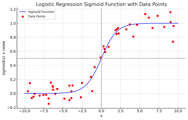
Logistic Regression: Logistic regression is a basic technique used for binary classification problems. In the context of anomaly detection, we could classify data as ‘normal’ or ‘anomaly’. Despite its simplicity, logistic regression can serve as a good starting point due to its interpretability and fast training times

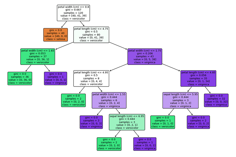
2. Decision Trees and Random Forests: Decision trees classify data by making decisions based on feature values, and they are easily interpretable. A random forest is an ensemble of decision trees which can give a more accurate and stable prediction. These can be used to identify anomalies if the anomalies cause the data to be classified differently.

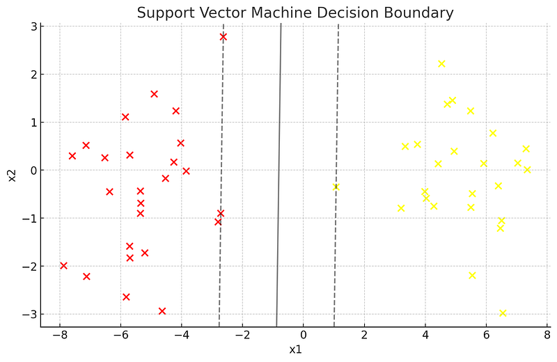
3. Support Vector Machines (SVMs): In the context of anomaly detection, SVMs can be used in a method known as One-Class SVM. This algorithm is trained on data representing only the normal state, differentiating new data points as either similar to the normal state (non-anomalous) or different (anomalous).

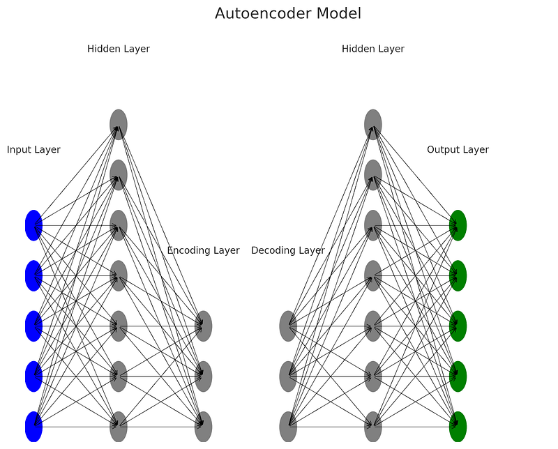
4. Neural Networks and Deep Learning: More complex models like neural networks can capture complex patterns in the data. A type of network called Autoencoders has gained popularity for anomaly detection. Autoencoders are trained to reconstruct their input data, and a high reconstruction error can indicate an anomaly. Convolutional Neural Networks (CNNs) and Recurrent Neural Networks (RNNs) can also be used for anomaly detection, especially with image and sequence data, respectively

Unsupervised Learning Algorithms for Anomaly Detection

Unsupervised learning algorithms do not require labeled data. They work by learning the normal patterns and identifying anomalies as deviations from these normal patterns.

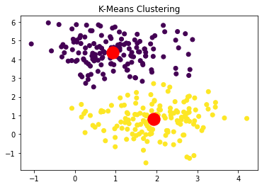
Clustering Algorithms: Clustering algorithms like K-means, DBSCAN, and Hierarchical Clustering group similar data points together. Data points that don’t fit into any cluster, or form small, separate clusters, can be considered anomalies.

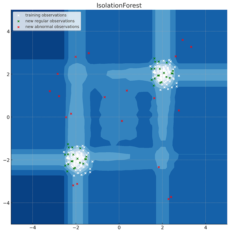
2. Outlier Detection Algorithms: Algorithms like Local Outlier Factor (LOF), Isolation Forest, and Elliptic Envelope are specifically designed for detecting outliers in the data. They each have a different approach, but essentially, they assign an ‘outlierness score’ to each data point, and data points with a score above a certain threshold are considered outliers.

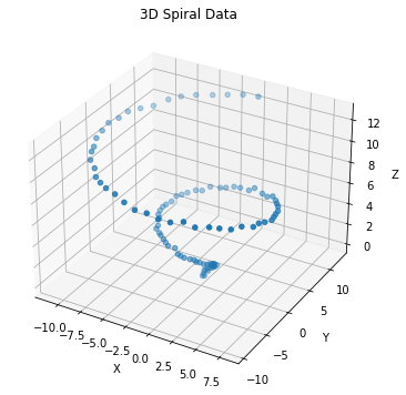
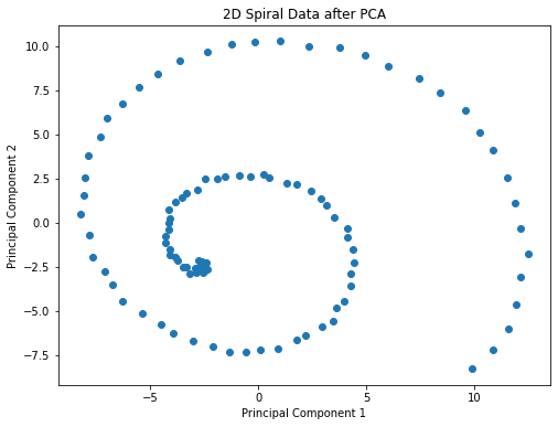
3. Principal Component Analysis (PCA): PCA is a dimensionality reduction technique that can be used for anomaly detection. It represents data in a lower-dimensional space, and anomalies are often detected as data points that have high reconstruction errors when represented by these principal components.

Semi-Supervised Learning Algorithms for Anomaly Detection

Semi-supervised learning algorithms use a small amount of labeled data and a large amount of unlabeled data.

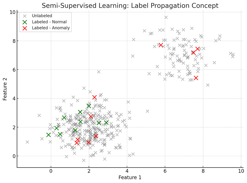
Label Spreading and Label Propagation: These methods begin with a small set of labeled instances and spread these labels to the unlabeled instances, using the data’s structure to guide the propagation.

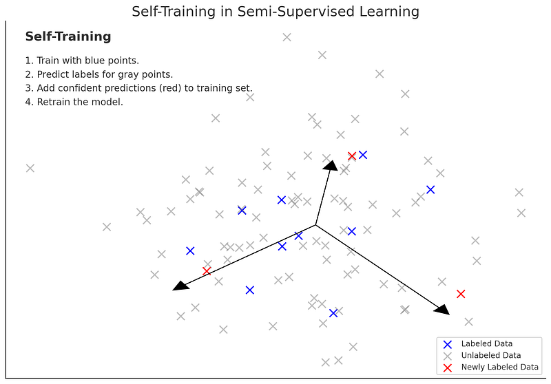
2. Self-Training: In self-training, a model is initially trained with a small set of labeled data, and then this model is used to predict labels for the unlabeled data. The most confident predicted labels are then added to the training set, and the model is retrained.

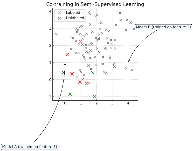
3. Co-training: In co-training, two models are trained independently on separate views of the data (i.e., different subsets of the features), and they label the unlabeled instances for each other. This process continues iteratively.

The choice of algorithm depends on the specific application, nature of the data, and available computational resources.

Coding Time: Supervised Learning with Logistic Regression

In this section, we will use a Supervised Learning method, specifically Logistic Regression, for anomaly detection. This technique will be employed on a synthetically generated dataset, which will contain two classes — ‘Normal’ and ‘Anomaly’. By performing Logistic Regression, we will attempt to classify whether a datapoint is normal or an anomaly.

The dataset we are utilizing here is generated using the make_classification function of Scikit-Learn, which creates a binary classification problem. In this problem, class ‘0’ is considered normal data and class ‘1’ signifies anomalies. To make the task more realistic and challenging, we are creating an imbalanced dataset, where anomalies constitute the minority class.

We will split the dataset into training and test sets. Then, we will train a Logistic Regression model using the training data and subsequently evaluate it on the test data, using a variety of performance metrics such as the confusion matrix, precision, recall, F1-score, and ROC AUC score.

import matplotlib.pyplot as plt
import pandas as pd
from sklearn.datasets import make_classification
from sklearn.model_selection import train_test_split
from sklearn.linear_model import LogisticRegression
from sklearn.metrics import classification_report, roc_auc_score
from sklearn.metrics import plot_confusion_matrix

# Generate the dataset
X, y = make_classification(n_samples=1000, n_features=20, n_informative=2, n_redundant=10,
                           n_clusters_per_class=1, weights=[0.99], flip_y=0, random_state=1)

# Print the data
print("Data:\n")
pd.DataFrame(X).head()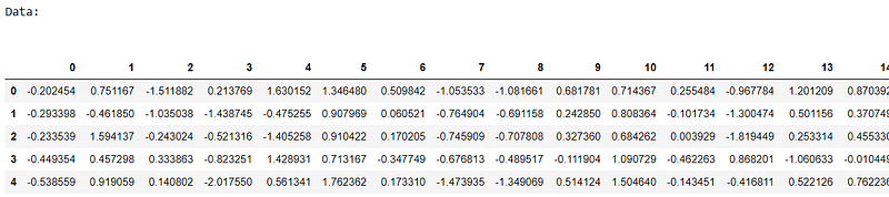

pd.DataFrame(y, columns=['Target'])['Target'].value_counts()

0 990 1 10 Name: Target, dtype: int64

# Plot the target variable
plt.hist(y, bins=2, rwidth=0.8)
plt.title("Distribution of the target variable")
plt.xticks([0,1])
plt.show()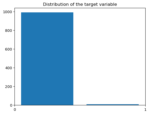

Next we use the `train_test_split` function from `sklearn` to divide the data into a training set and a test set. `X` and `y` represent the features and the target variable respectively. The `test_size=0.2` specifies that 20% of the data is reserved for the test set, while the rest is used for training. The `random_state=42` ensures reproducibility of results by providing a seed to the random number generator for shuffling the data before splitting.

# Split the dataset into training and test datasets
X_train, X_test, y_train, y_test = train_test_split(X, y, test_size=0.2, random_state=42)

Next, we create and train a logistic regression model using the scikit-learn library. The `LogisticRegression()` function initiates the logistic regression model, and the `solver=’liblinear’` argument specifies the algorithm to use for optimization problem, `liblinear` is particularly suitable for small datasets.

The `model.fit(X_train, y_train)` line is where the training process happens. The `fit` function adjusts the model’s internal parameters to minimize the cost function (which measures the discrepancy between the model’s predictions and the actual data). It takes the features `X_train` and the corresponding targets `y_train` from the training dataset as inputs and then adjusts the model’s parameters to find the best fit that can predict the target variable from the features. This is achieved through an iterative process of learning from the data in the training set.

# Train a logistic regression model
model = LogisticRegression(solver='liblinear')
model.fit(X_train, y_train)

After training the model, we are going to use it to make predictions on the test set.

# Predict the test set results
y_pred = model.predict(X_test)
y_pred_proba = model.predict_proba(X_test)[:, 1]

`y_pred = model.predict(X_test)`: This line uses the `predict` function of the trained model to predict the target variable (`y`) for the test set (`X_test`). The `predict` function returns the predicted class labels — in this case, it would return 0 for normal data and 1 for an anomaly.

`y_pred_proba = model.predict_proba(X_test)[:, 1]`: This line uses the `predict_proba` function to predict the probability estimates for the test set (`X_test`). This function returns the probability of the sample for each class in the model. The output is a two-column array where the first column contains the probability that a sample is a member of the first class and the second column contains the probability that a sample is a member of the second class. We are only interested in the second column, i.e., the probability that the data point is an anomaly, so we specify `[:, 1]` to select this column.

With our predictions, we can assess the performance of the model over unseen data:

# Evaluate the model
print("Classification Report: \n", classification_report(y_test, y_pred))
print("ROC AUC Score: ", roc_auc_score(y_test, y_pred))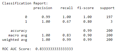

The classification report provides a detailed view of the performance of the logistic regression model for each class. It includes the following metrics:

1. Precision: This is the ratio of correctly predicted positive observations to the total predicted positives. High precision relates to a low false positive rate. It is also known as Positive Predictive Value (PPV).

2. Recall (Sensitivity): This is the ratio of correctly predicted positive observations to all observations in the actual class. High recall relates to a low false negative rate.

3. F1 Score: This is the weighted average of Precision and Recall. It tries to find the balance between precision and recall.

4. Support: This is the number of actual occurrences of the class in the specified dataset. For instance, in our binary classification problem, it would tell us how many instances of normal data points (class 0) and anomalies (class 1) exist in the test set.

The reported averages include macro average (averaging the unweighted mean per label), weighted average (averaging the support-weighted mean per label), and sample average (only for multilabel classification). ‘Micro average (averaging the total true positives, false negatives and false positives)’ is only shown for multi-label or multi-class with a subset of classes because it corresponds to accuracy otherwise.

High values for these metrics are desirable, indicating that the model is doing a good job of distinguishing between normal data points and anomalies.

The `roc_auc_score` function computes the area under the receiver operating characteristic (ROC) curve, which is a graphical representation of the performance of a classification model. The ROC curve plots the true positive rate (sensitivity) against the false positive rate (1 — specificity), and the area under the curve (AUC) represents the degree of separability achieved by the model. An AUC score closer to 1 indicates that the model is able to distinguish between normal data points and anomalies effectively, whereas a score closer to 0.5 suggests the model is performing no better than random chance.

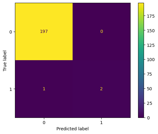
The confusion matrix is a summary of the predictions made by a classification algorithm. It’s a table with two dimensions: “Predicted” and “Actual”. In binary classification, the two dimensions of the table can be labeled as “Positive” (the event happened, or “yes”) and “Negative” (the event did not happen, or “no”).

Here’s a brief explanation of each term:

1. True Positives (TP): These are cases in which we predicted “yes” (or positive), and the actual result was also “yes”.

2. True Negatives (TN): We predicted “no” (or negative), and the actual result was “no”.

3. False Positives (FP): We predicted “yes”, but the actual result was “no”. This is also known as a “Type I error” or “False Alarm”.

4. False Negatives (FN): We predicted “no”, but the actual result was “yes”. This is also known as a “Type II error” or “Miss”.

Here’s a visual representation of a confusion matrix for a binary classification problem:

This matrix provides a lot of information, but sometimes we might want to boil it down to a single metric for comparison purposes. Several such metrics can be computed from a confusion matrix, such as precision, recall, and F1-score which are part of the classification report we discussed before.

Interpretation of Results

The dataset used in this example was synthetically generated using the `make_classification` function from the Scikit-learn library for demonstration purposes, and so, the data and results are illustrative rather than indicative of a specific real-world situation. This tool is valuable for demonstrating concepts, testing methodologies, or benchmarking algorithms in a controlled manner.

Looking at the performance metrics, we can conclude that our logistic regression model was able to successfully identify anomalies in this controlled environment. However, it’s important to remember that results might not translate directly to a real-world dataset, where the distribution, number, and complexity of anomalies can be much more diverse and unpredictable.

The model showed excellent precision, suggesting that it correctly identified almost all of the normal transactions (class 0) and all anomalous transactions (class 1) when it predicted them. This is a critical aspect in anomaly detection scenarios as false positives can lead to wasted resources.

On the other hand, the recall for anomalous transactions was lower, indicating that the model missed a third of the actual anomalies. This indicates a limitation in our model’s ability to detect all anomalies and shows the challenge of dealing with imbalanced datasets typical of anomaly detection tasks.

The ROC AUC Score was relatively high, suggesting our model was effective in distinguishing between normal and anomalous transactions, though there’s room for improvement.

Overall, the logistic regression model provided a strong baseline for anomaly detection in this illustrative dataset. However, in practice, you might need to explore more sophisticated methods or ensemble techniques to improve the detection of anomalous transactions. Also, remember to tune the model and adjust the threshold according to the specific requirements and constraints of your real-world project.

Coding Time: Supervised Learning with Decision Tree Classifiers

For this section, we will demonstrate how to apply a Decision Tree Classifier for classification. Decision Trees are simple yet powerful machine learning algorithms. They can capture complex patterns in the data by splitting the data based on the values of the features. The features to split on and the split points are chosen to maximize the separation of the classes.

We will use the Iris dataset in this example, a classic dataset often used for classification tasks. It includes measurements of 150 iris flowers from three different species — Setosa, Versicolour, and Virginica. Each instance includes four measurements: sepal length, sepal width, petal length, and petal width. In the context of anomaly detection, one could consider the instances of a particular species as “normal” and the instances of the other species as “anomalies”.

First, we will load and explore the dataset. Then, we will divide the data into training and testing datasets. We will then train a Decision Tree Classifier on the training data and evaluate its performance on the testing data using a variety of performance metrics.

import pandas as pd
from sklearn.model_selection import train_test_split
from sklearn.tree import DecisionTreeClassifier
from sklearn.metrics import classification_report, roc_auc_score, plot_confusion_matrix
from sklearn.datasets import load_iris
import matplotlib.pyplot as plt

# Load the iris dataset
iris = load_iris()
X = iris.data
y = iris.target

# Print the data
print("Data:\n")
pd.DataFrame(X, columns=iris.feature_names).head()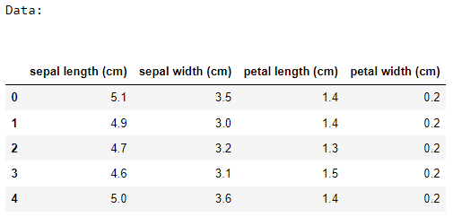

pd.DataFrame(y, columns=['Species'])['Species'].value_counts()

0 50 1 50 2 50 Name: Species, dtype: int64

# Plot the target variable
plt.hist(y, bins=3, rwidth=0.8)
plt.title("Distribution of the Species")
plt.xticks([0,1,2], iris.target_names)
plt.show()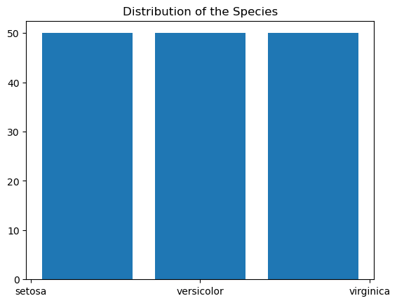

# Split the dataset into training and test datasets
X_train, X_test, y_train, y_test = train_test_split(X, y, test_size=0.2, random_state=42)

# Train a Decision Tree Classifier
model = DecisionTreeClassifier()
model.fit(X_train, y_train)

# Predict the test set results
y_pred = model.predict(X_test)
y_pred_proba = model.predict_proba(X_test)

# Evaluate the model
print("Classification Report: \n", classification_report(y_test, y_pred))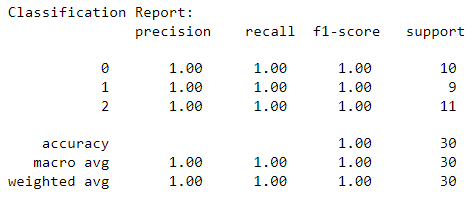

# Plot the confusion matrix
plot_confusion_matrix(model, X_test, y_test)
plt.show()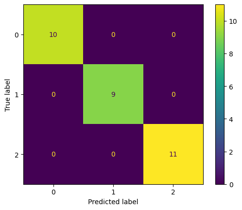

The subsequent steps of splitting the data, training the model, predicting the test results, and evaluating the model are very similar to the previous Logistic Regression example. The difference lies in the model we are using, which is a Decision Tree Classifier in this case.

Now you can compare the performance of the Decision Tree Classifier to the Logistic Regression model from the previous section. Does the Decision Tree Classifier perform better or worse? How does the nature of the dataset affect the performance of the different algorithms?

These are some of the questions you can explore further as you dive deeper into anomaly detection with supervised learning methods.

The structure of the decision tree can be visualized using libraries like matplotlib and sklearn.tree. Here is an example of how you can plot the tree:

from sklearn.tree import plot_tree

# Plot the decision tree
plt.figure(figsize=(15,10))
plot_tree(model, 
          filled=True, 
          rounded=True, 
          class_names=iris.target_names, 
          feature_names=iris.feature_names)
plt.show()

In this code, plot_tree is used to plot the decision tree. The filled=True argument fills the boxes representing the tree nodes with colors, and rounded=True makes the corners of the boxes rounded. class_names=iris.target_names provides the names of the classes and feature_names=iris.feature_names provides the names of the features.

This visualization can give you a detailed view of how the decision tree makes predictions. Each node of the tree splits the data based on a condition on one of the features, and the tree continues to split the data until it reaches a condition where it can make a confident prediction. This process is represented by the tree structure, where the root is the initial split and the leaves are the final predictions.

You can control the depth of the decision tree by setting the max_depth parameter when you create the DecisionTreeClassifier object. This parameter determines the maximum depth of the tree. Limiting the depth of the tree can make your model simpler and easier to interpret, and can also help prevent overfitting.

Here’s how you can limit the depth of your tree:

model = DecisionTreeClassifier(max_depth=3)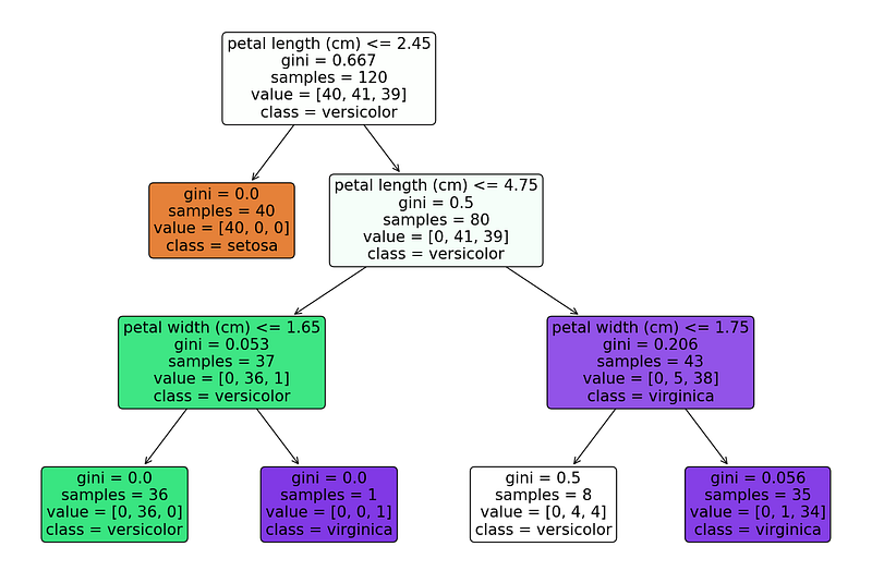

We’ll continue from here in Part 2 of Chapter 3!

Link to Chapter 3 code: https://github.com/gabrielpierobon/anomaly_detection/blob/main/Chapter%2003%20Introduction%20to%20Machine%20Learning%20for%20Anomaly%20Detection.ipynb

Link to PDF Guide: https://drive.google.com/file/d/1g77lB2zeZGQUqIyPSb9Fr-uMyjmAG4j4/view?usp=drive_link