DBSCAN for Anomaly detection

A carefully generated, thoroughly engineered resource for Data Scientists.

Chapter 06 from the Guide to Machine Learning for Anomaly Detection

I actually wrote a full article con DBSCAN some years ago, but not focused on anomaly detection.

Warning! Before you continue reading this article and all the articles that compose this guide, you must understand this was in part generated using OpenAI’s GPT 4 model. It started as a self learning project and I soon enough realized this could be really valuable to fellow data scientists. Because of this, I will release the entire guide for free alongside every chapter so you can directly go read the guide from the document so you don’t even need to give me reading time if you don’t want to.

Guide Index

The quest to understand and make sense of large, complex datasets has brought forth a plethora of machine learning algorithms and techniques, each with its unique strengths and trade-offs. As we explored in the previous chapters, we began our journey into the realm of anomaly detection by utilizing supervised learning algorithms. We further delved into unsupervised learning, particularly partitioning-based clustering methods, with K-Means serving as our tool of choice.

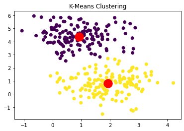
Despite the success of K-Means, it has its limitations; mainly its difficulty to handle noise and outliers, and its assumption of spherical clusters. These restrictions can be important, especially in real-world applications where data may not conform to such ideal conditions.

Chapter 6 marks a shift in our approach.

We will explore a new technique that doesn’t merely partition data into clusters but takes into account the spatial density of data points — DBSCAN (Density-Based Spatial Clustering of Applications with Noise).

DBSCAN’s strength lies in its ability to identify clusters of various shapes and sizes, and its resilience to noise and outliers, thereby making it a potent tool for anomaly detection. In this chapter, we will unpack DBSCAN, its workings, and its application in detecting anomalies in complex datasets.

Understanding DBSCAN: Intuition and Concepts

The concept behind DBSCAN (Density-Based Spatial Clustering of Applications with Noise) is in its name itself — it’s a density-based clustering algorithm. Unlike K-Means, which partitions data into spherical clusters and can misinterpret outliers as small clusters, DBSCAN locates regions of high density and separates them from regions of low density.

This unique characteristic allows it to discover clusters of arbitrary shapes and sizes and handle noise and outliers, making it particularly suitable for anomaly detection.

Let’s break down the intuition behind DBSCAN:

Density

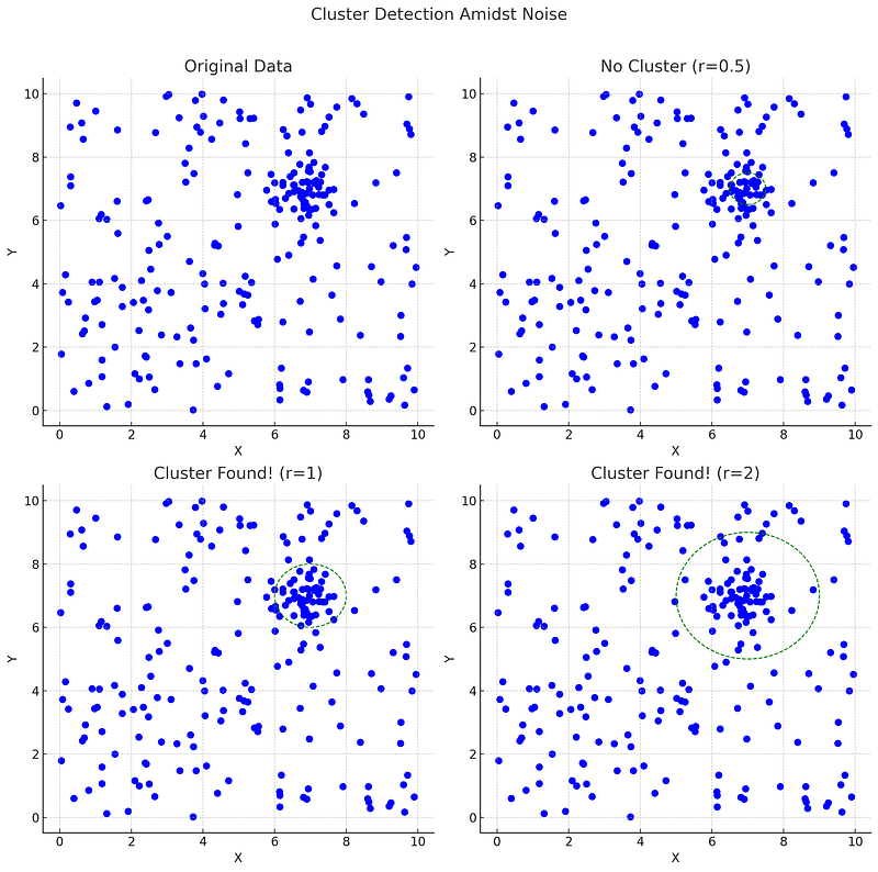
At its core, DBSCAN classifies data points based on the area density around them. If a specific area has enough points (defined by a parameter), DBSCAN considers it as a cluster.

A DBSCAN-alike approach. The top-left plot shows the original data with all points in blue .The other three plots demonstrate the cluster detection process using circles of radii 0.50.5, 11, and 22.

Reachability

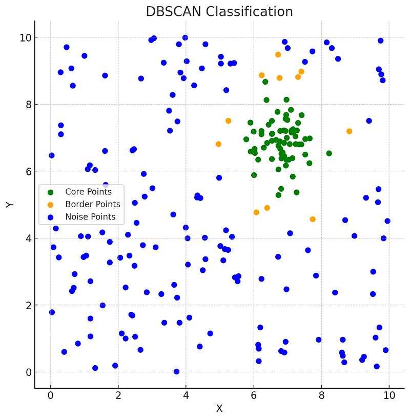
DBSCAN classifies points into three categories:

core points
border points
noise points

Core points are those that have a minimum number of points (MinPts) within a specified radius ε. Border points have fewer than MinPts within ε but are in the neighborhood of a core point. Noise points are all other points that are neither core nor border points.

Connectivity

If a point is reachable from another, and the latter is a core point, they belong to the same cluster. DBSCAN starts with an arbitrary core point, clusters all directly reachable points, and continues the process recursively, resulting in a density-connected cluster.

Here’s an illustration showcasing the reachability concept of DBSCAN:

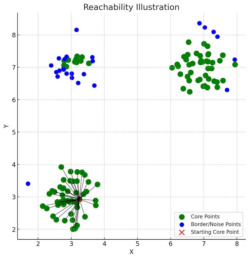
Green Points: These are the core points. A core point has at least MinPts neighbors within the radius ε.
Blue Points: These are either border points or noise points.
Red “X” Mark: This indicates our starting arbitrary core point.

The black lines drawn from the starting core point to other core points represent the concept of reachability. If a point is reachable from the starting point within the radius ε and is a core point, they belong to the same cluster.

By starting from a core point and continuing this process recursively with all reachable core points, DBSCAN forms a density-connected cluster.

In contrast to partitioning-based methods, DBSCAN doesn’t require the user to specify the number of clusters a priori. It determines the clusters based on the dataset’s intrinsic structure. This feature makes DBSCAN a more flexible and robust choice for datasets with complex structures.

In the next sections, we’ll dive deeper into DBSCAN’s working mechanism and apply it to real-world datasets for anomaly detection.

Coding Time: DBSCAN

The objective of this exercise is to showcase the efficiency of DBSCAN in identifying arbitrary shaped clusters and its application in anomaly detection. We will use a synthetic Moons dataset for this purpose.

The Moons dataset is a synthetic dataset that is part of Scikit-learn’s datasets module. It consists of two interleaved half-circle shapes. We will introduce just a little bit of noise in the data to demonstrate DBSCAN’s ability to ignore outliers and focus on the denser areas of the feature space.

# Import necessary libraries
from sklearn.datasets import make_moons
import matplotlib.pyplot as plt
import seaborn as sns

# Generate the moon dataset with noise
X, y = make_moons(n_samples=500, noise=0.05, random_state=42)

# Visualize the dataset
plt.figure(figsize=(8, 5))
sns.scatterplot(x=X[:,0], y=X[:,1])
plt.title('Moons Dataset')
plt.show()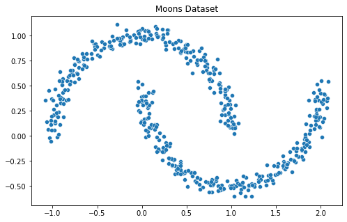

This is a weird looking set of points, and this is what happens when we try to use K-Means to find the clusters:

# Import necessary libraries
from sklearn.cluster import KMeans

# Define the K-Means model
kmeans = KMeans(n_clusters=2, random_state=42)

# Fit the model
kmeans.fit(X)

# Predict the cluster labels
labels_kmeans = kmeans.predict(X)

# Visualize the K-Means clustering result
plt.figure(figsize=(8, 5))
sns.scatterplot(x=X[:,0], y=X[:,1], hue=labels_kmeans, palette='viridis')
plt.scatter(kmeans.cluster_centers_[:,0], kmeans.cluster_centers_[:,1], color='red', label='Centroids')
plt.title('K-Means Clustering on Moons Dataset')
plt.legend()
plt.show()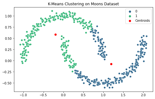

Clearly K-Means can’t do a good job with these representations. So we’ll now move on to DBSCAN:

# Import necessary libraries
from sklearn.cluster import DBSCAN

# Define the DBSCAN model
dbscan = DBSCAN(eps=0.3, min_samples=5)

# Fit the model and predict the cluster labels
labels_dbscan = dbscan.fit_predict(X)

# Visualize the DBSCAN clustering result
plt.figure(figsize=(8, 5))
sns.scatterplot(x=X[:,0], y=X[:,1], hue=labels_dbscan, palette='viridis')
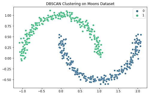
plt.title('DBSCAN Clustering on Moons Dataset')
plt.show()

Impressive!

In the above code, we create a DBSCAN model with an epsilon (eps) of 0.3 and a minimum samples (min_samples) of 5. These parameters determine the maximum distance between two samples for one to be considered as in the neighborhood of the other, and the number of samples in a neighborhood for a point to be considered as a core point, respectively. Adjusting these parameters will affect the result of the clustering.

The DBSCAN algorithm successfully identifies the two moon-shaped clusters, demonstrating its effectiveness on this kind of dataset. Unlike K-Means, DBSCAN does not assume that clusters are spherical, and thus can accurately identify clusters of arbitrary shapes.

Can DBSCAN find anomalies/outliers in a dataset?

Yes!,

DBSCAN can be used for anomaly detection in addition to clustering.

One of the distinguishing features of DBSCAN is that, as I mentioned above, it separates data points into three types: core points, border points, and noise points.

As we have already seen:

Core points are points that have at least a specified number (min_samples) of neighboring points within a given distance (eps). These are interpreted as points that are in a dense region of the feature space, and they form the main body of a cluster.
Border points are points that have fewer than min_samples within eps, but are in the neighborhood of a core point. These points are on the edges of a cluster.
Noise points, also known as outliers, are points that are neither core points nor border points. These points could be interpreted as anomalies. They are assigned the cluster label -1 by the DBSCAN algorithm.

So, in a sense, DBSCAN inherently includes an anomaly detection step in its process.

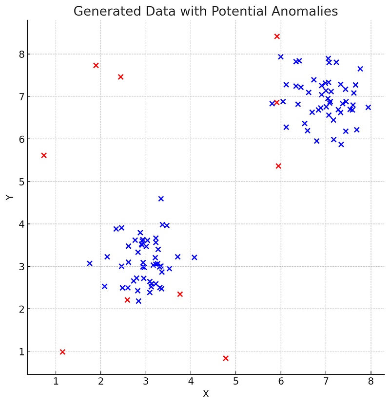
After running DBSCAN, you can isolate the noise points and study them to understand why the algorithm identified them as anomalies. This makes DBSCAN a handy tool for both clustering and anomaly detection, particularly when you expect the anomalies to be scattered randomly and not part of smaller clusters.

Coding Time: Anomaly Detection with DBSCAN

In this section, we will demonstrate how to use DBSCAN for anomaly detection on the credit card fraud dataset. Our objective is to identify unusual transactions, which could potentially be fraudulent.

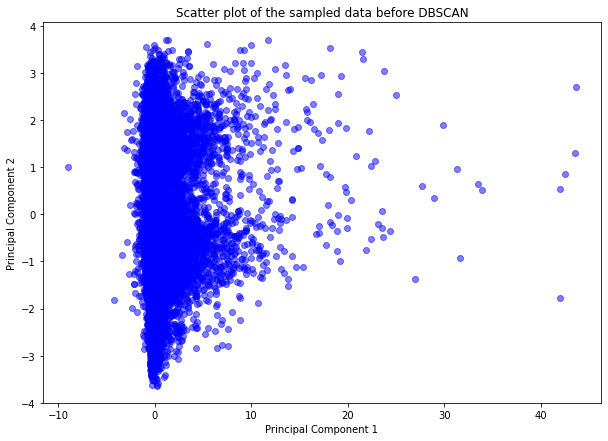
Let’s continue from where we left off in our previous chapter. We have already loaded the data but we will sample from it because DBSCAN takes too much compute time to process. We separated the features and labels, standardized the features, and applied PCA to reduce dimensions.

from sklearn.cluster import DBSCAN

# Define the DBSCAN model
dbscan = DBSCAN(eps=0.3, min_samples=5)

# Fit and predict the labels
labels = dbscan.fit_predict(X_pca)

# Identify the core and outlier samples
core_samples_mask = np.zeros_like(dbscan.labels_, dtype=bool)
core_samples_mask[dbscan.core_sample_indices_] = True
labels = dbscan.labels_

# Get the number of clusters (ignoring noise if present)
n_clusters_ = len(set(labels)) - (1 if -1 in labels else 0)
n_noise_ = list(labels).count(-1)

print(f'Estimated number of clusters: {n_clusters_}')
print(f'Estimated number of noise points: {n_noise_}')

# Plot the data, color code by DBSCAN cluster assignment
plt.figure(figsize=(10,7))
unique_labels = set(labels)
colors = [plt.cm.Spectral(each) for each in np.linspace(0, 1, len(unique_labels))]
for k, col in zip(unique_labels, colors):
    if k == -1:
        col = [0, 0, 0, 1]  # Black used for noise.
    class_member_mask = (labels == k)

    xy = X_pca[class_member_mask & core_samples_mask]
    plt.plot(xy[:, 0], xy[:, 1], 'o', markerfacecolor=tuple(col), markeredgecolor='k', markersize=14)

    xy = X_pca[class_member_mask & ~core_samples_mask]
    plt.plot(xy[:, 0], xy[:, 1], 'o', markerfacecolor=tuple(col), markeredgecolor='k', markersize=6)
plt.title(f'Estimated number of clusters: {n_clusters_}')
plt.xlabel('Principal Component 1')
plt.ylabel('Principal Component 2')
plt.show()

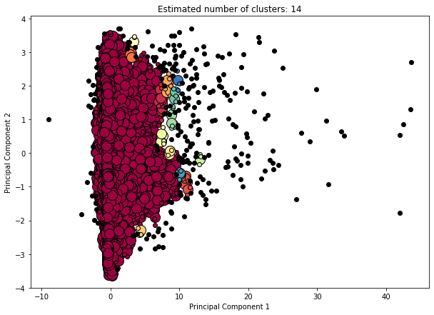
Estimated number of clusters: 14 Estimated number of noise points: 251

Results

Estimated number of clusters: 14

DBSCAN has identified 14 separate clusters in our data.
Means that the algorithm has found 14 distinct groups of data points where each group’s points are densely packed together in the feature space.

Estimated number of noise points: 251

DBSCAN has marked 251 data points as noise.
These are points that do not belong to any cluster because they are not part of a dense region.

In DBSCAN, noise points could either be anomalies/outliers or points that reside between clusters.

In this context, these noise points can potentially be considered as anomalies or outliers. However, be careful with this interpretation as not all noise points are true anomalies. We might need further analysis to confirm.

DBSCAN labels noise points as -1 and assigns other positive integers for different clusters. So, in this case, our dataset has data points belonging to 14 different clusters and 251 points that couldn’t be assigned to any cluster and hence, are considered noise.

We can compare our results with the real classes from the data:

# Create a cross-tabulation table
crosstab = pd.crosstab(data_sample['Class'], data_sample['anomaly'])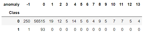

The cross table shows the distribution of the original class labels (Class) across the different clusters identified by DBSCAN (represented by the anomaly column).

Here’s how you can interpret it:

Cluster -1

This is the cluster representing noise or outliers as per DBSCAN. There are 250 instances from the original class 0 (the majority class) and 1 instance from the original class 1 (the minority class) in this cluster. The fact that this cluster contains an instance from the minority class could indicate that DBSCAN identified it as an anomaly.

Cluster 0

This cluster is the largest and contains 56515 instances from the original class 0 and 93 instances from the original class 1. Most of the data points are included in this cluster, which suggests it’s likely representing normal behavior in the data.

Clusters 1 to 13

These clusters represent smaller groups of instances exclusively from the original class 0. Each of these clusters could represent some specific characteristic of the data where instances from the majority class are densely packed together. However, since no instances from the minority class are found in these clusters, they probably don’t represent fraudulent behavior.

It’s important to note that the size and composition of these clusters greatly depend on the choice of parameters in DBSCAN. We might need to adjust the eps and min_samples parameters to achieve better anomaly detection results, particularly for identifying instances from the minority class.

Also, keep in mind that cluster analysis, like DBSCAN, is not designed primarily for class separation. It’s an exploratory data analysis tool used to identify structure in unlabeled data. Therefore, don’t be surprised if the clustering results don’t perfectly align with the original class labels.

That being said, the results here show that DBSCAN has some potential in identifying anomalies within the dataset.

See you in Chapter 7!

Code for Chapter 6: https://github.com/gabrielpierobon/anomaly_detection/blob/main/Chapter%2006%20DBSCAN%20for%20anomaly%20detection.ipynb

Link to PDF Guide: https://drive.google.com/file/d/1g77lB2zeZGQUqIyPSb9Fr-uMyjmAG4j4/view?usp=drive_link