K-Nearest Neighbors (KNN) for Anomaly Detection
A carefully generated, thoroughly engineered resource for Data Scientists.
Chapter 09 from the Guide to Machine Learning for Anomaly Detection
Warning! Before you continue reading this article and all the articles that compose this guide, you must understand this was in part generated using OpenAI’s GPT 4 model. It started as a self learning project and I soon enough realized this could be really valuable to fellow data scientists. Because of this, I will release the entire guide for free alongside every chapter so you can directly go read the guide from the document so you don’t even need to give me reading time if you don’t want to.

Guide Index
0: About the generation of this guide 1: Introduction to Anomaly Detection 2: Statistical Techniques for Anomaly Detection (Part 1) 2: Statistical Techniques for Anomaly Detection (Part 2) 3: Introduction to M. Learning for Anomaly Detection (Part 1) 3: Introduction to M. Learning for Anomaly Detection (Part 2) 4: Dealing with Imbalanced Classes in Supervised Learning 5: K-Means Clustering for Anomaly detection 6: DBSCAN for Anomaly detection 7: Isolation Forest for Anomaly Detection 8: One-Class SVM for Anomaly Detection >>>>> 9: K-Nearest Neighbors (KNN) for Anomaly Detection <<<<< 10: Principal Graph and Structure Learning (PGSL) for Anomaly Detection 11: Dimensionality Reduction Techniques for Anomaly Detection 12: Singular Value Decomposition (SVD) for Anomaly Detection 13: Advanced Matrix Factorization Techniques for Anomaly Detection 14: Nystrom Method for Anomaly Detection 15: Kernel Methods for Anomaly Detection 16: Advanced Algorithms for Anomaly Detection 17: Feature Selection and Engineering for Anomaly Detection 18: Semi-Supervised Learning for Anomaly Detection 19: Deep Learning for Anomaly Detection 20: Ensemble Methods for Anomaly Detection 21: Evaluation Metrics for Anomaly Detection 22: Case Studies and Industry Applications 23: Conclusion and Future Directions in Anomaly Detection
After an extensive exploration of statistical and machine learning methods like z-scores, DBSCAN, Isolation Forests, and One-Class SVM, we arrive at an algorithm that is both intuitive and remarkably effective: K-Nearest Neighbors (KNN).
The KNN algorithm, in the realm of machine learning, is somewhat of a jack-of-all-trades, with applications in classification, regression, and as we will focus on in this chapter, anomaly detection. KNN’s simplicity in concept, versatility, and robustness have contributed to its enduring popularity.
It’s an instance-based, lazy learning algorithm, which means it doesn’t explicitly learn a model. Instead, it memorizes the training instances and uses them for prediction.
The premise of KNN for anomaly detection is simple: a data point is considered an anomaly if its environment, defined by its K-nearest neighbors, significantly deviates from the environment of other data points in the dataset.
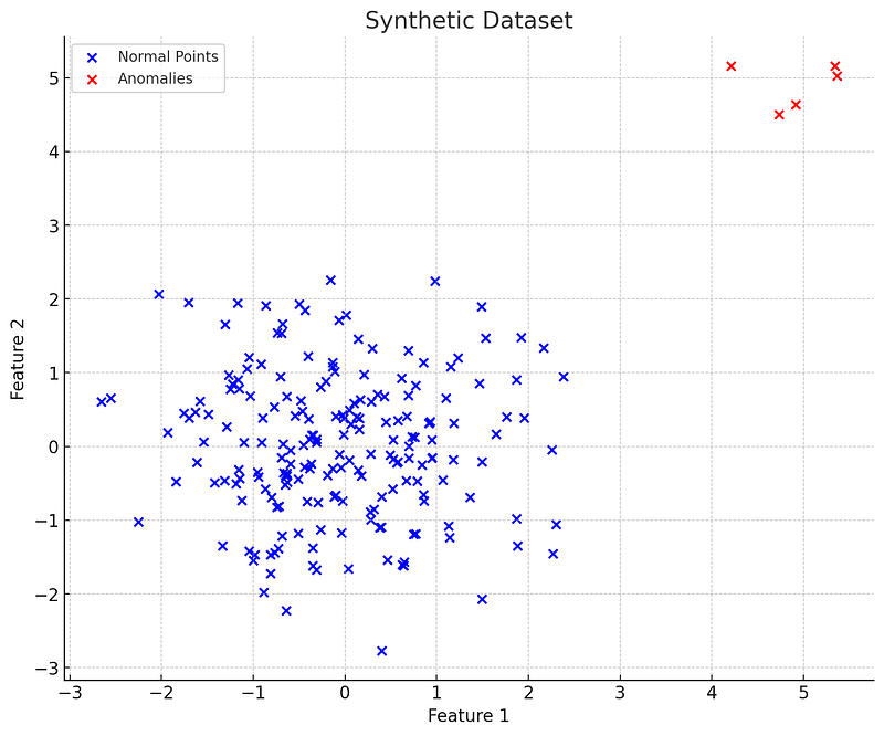
This concept hinges on the idea of distance metrics, which quantify the dissimilarity between data points. This approach makes KNN a particularly suitable choice for datasets with complex structures, where anomalies are not necessarily outliers but instead, objects that don’t comply with the usual patterns or structures in the data.
However,
the success of KNN also hinges on the careful selection of hyperparameters, the most critical being the number of neighbors ‘K’, and the choice of the distance metric.
They both significantly influence the algorithm’s performance and the quality of results.
In this chapter, we will delve into the intricacies of KNN, starting with an overview of the algorithm. We’ll delve into the importance of distance metrics and the role they play in determining neighbors. We will then explore how KNN is used for anomaly detection, both in theory and practice. As with the previous chapters, we will bring these concepts to life through Python implementation on both synthetic and real-world datasets.
KNN Overview
The K-Nearest Neighbors (KNN) algorithm is a non-parametric method used for classification, regression, and anomaly detection. It’s based on feature similarity, meaning it classifies a new object based on how closely it resembles the objects in the training set.
The intuition behind the KNN algorithm is quite straightforward: “Like attracts like”. In essence,
similar things exist in close proximity.
For instance, if you’re searching for a restaurant in a city, you’ll likely find several of them clustered in certain districts.

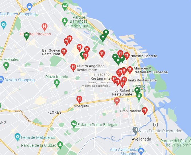
The same principle is applied in the KNN algorithm, where we predict the class or value of a data point based on the classes or values of the data points in its vicinity.
Here are the basic steps of the KNN algorithm:
- Choose the number of neighbors (K): The first step in the KNN algorithm is to determine the ‘K’ value, which represents the number of nearest neighbors we’ll look at. K is usually an odd number if the number of classes is 2.
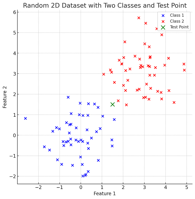
2. Find the K nearest neighbors: For each point, calculate the distance to all other points. Then select the K points that are nearest to the current point. The distance can be calculated in various ways, including Euclidean, Manhattan, Minkowski, or Hamming distance.
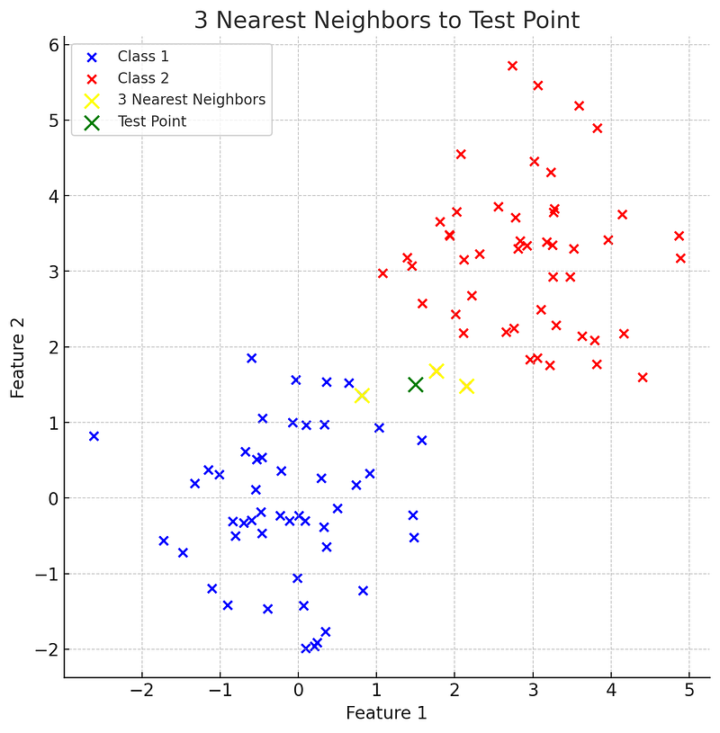

3. Majority voting (for classification): Once the K nearest neighbors are identified, we use them to make our prediction. In a classification context, we assign the class that is most common among the neighbors.
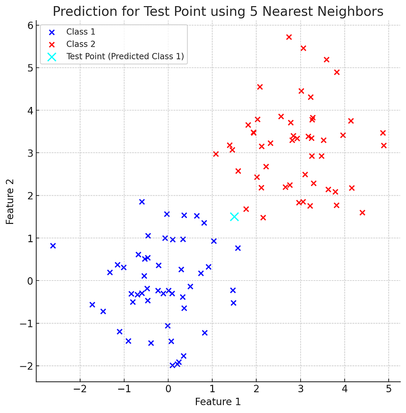
4. Calculate the mean (for regression): For regression problems, we can calculate the average of the K nearest neighbors to give the predicted value for the new data point.
5. Anomaly detection: For anomaly detection, a data point is flagged as an anomaly if it significantly deviates from the majority of its K nearest neighbors.
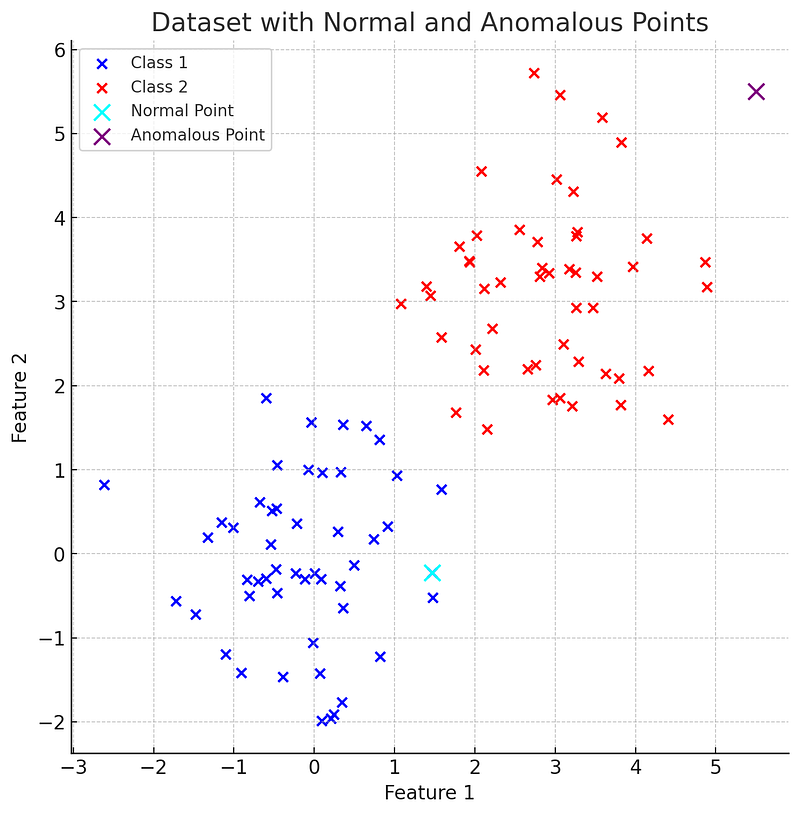
A crucial aspect of the KNN algorithm is its “laziness”.
It’s a lazy learning algorithm because it doesn’t learn a discriminative function from the training data but memorizes the training dataset instead.
The real computational work of the algorithm starts when it’s time to classify a new data point. Because of this, KNN can be computationally expensive and slow if you have a large amount of data.
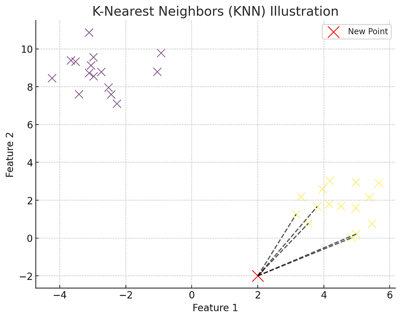
In this illustration, we have two types of data points represented by different colors. We introduce a new data point (represented by the red color). The five dashed lines represent the five nearest neighbors to this new data point.
By examining these nearest neighbors, the KNN algorithm will classify the new data point. In this case, the new point is classified as belonging to class 1, since the majority of its five nearest neighbors belong to this class.
Distance Metrics
Choosing the right distance metric is an essential step in the KNN algorithm, as it defines how we measure the nearness between data points. Different distance metrics may give different nearest neighbors and can significantly influence the algorithm’s performance. Here are some of the most commonly used distance metrics in the context of the KNN algorithm:
Euclidean Distance
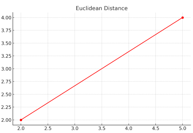
The Euclidean distance is the “ordinary” straight-line distance between two points in Euclidean space. With this distance, the KNN algorithm is also known as the Euclidean KNN classifier.
The Euclidean distance between two points `p` and `q` in a `n`-dimensional space is calculated as:
d(p, q) = sqrt[(p1-q1)² + (p2-q2)² + … + (pn-qn)²]
Manhattan Distance
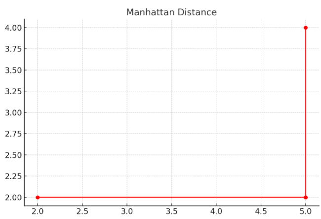
Also known as city block distance, Manhattan distance is the distance between two points in a grid-based system (like Manhattan street grid). It’s calculated as the sum of the absolute differences of their Cartesian coordinates. In contrast to Euclidean distance, Manhattan distance can move in orthogonal (right-angle) directions only.
The Manhattan distance between two points `p` and `q` in a `n`-dimensional space is calculated as:
d(p, q) = |p1-q1| + |p2-q2| + … + |pn-qn|
Minkowski Distance
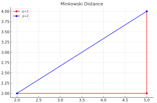
The Minkowski distance is a generalized metric form of Euclidean Distance and Manhattan Distance. By changing the value of `p` in the Minkowski equation, we can switch between Euclidean and Manhattan distances. In other words, Minkowski distance is a parameterized distance metric.
The Minkowski distance between two points `p` and `q` in a `n`-dimensional space is calculated as:
d(p, q) = (|p1-q1|^p + |p2-q2|^p + … + |pn-qn|^p)^(1/p)
Where `p` is the parameter:
* `p = 1` : Manhattan Distance
* `p = 2` : Euclidean Distance
Hamming Distance
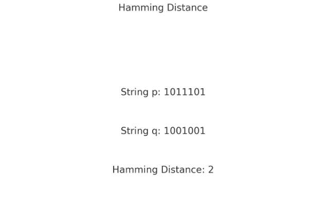
Hamming distance measures the minimum number of substitutions needed to change one string into the other or the minimum number of errors that could have transformed one string into the other. In the context of KNN, it is often used when dealing with categorical variables.
The distance metric you choose should reflect the nature of your data. For instance, if you’re working with high-dimensional data, you might want to consider the Euclidean distance or the Cosine similarity. If you’re dealing with binary or categorical data, the Hamming distance could be a good choice. It’s always a good idea to experiment with different distance metrics and see what works best for your specific use case.
Anomaly Detection with KNN
Having discussed the fundamentals of KNN and the various distance metrics used, we can now delve into how KNN is used for anomaly detection.
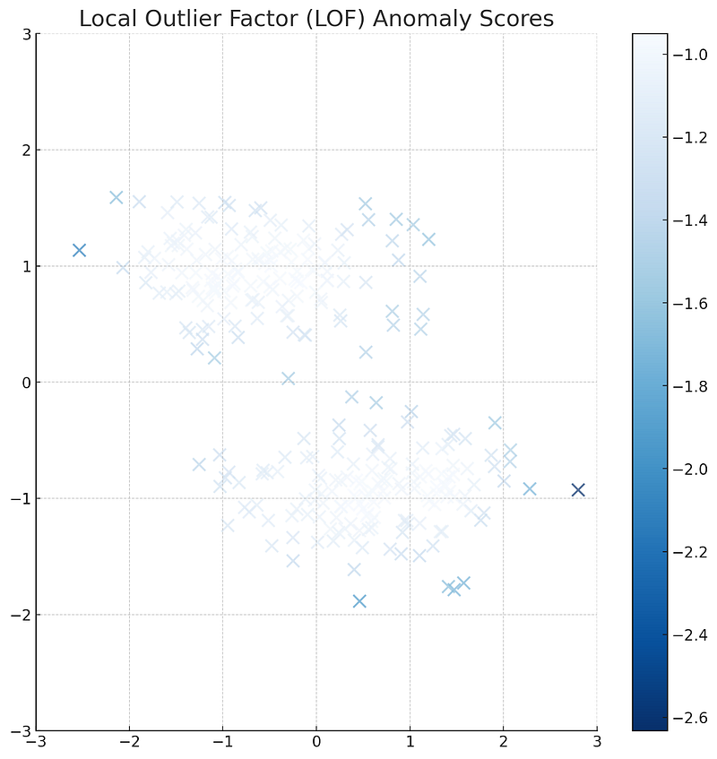
The principle behind KNN for anomaly detection is relatively straightforward. For a given data point, we calculate its distance to its nearest `k` neighbors. If this distance is significantly larger than the average distance of the majority of points in the dataset, the data point is considered an anomaly. This is under the assumption that normal data points occur close to each other while anomalies are far away.
Steps
- Standardization: Before applying the KNN algorithm, it’s often recommended to standardize your dataset so that all features contribute equally to the distance computation.
- Choosing `k`: The number of neighbors to consider (`k`) plays a crucial role in the performance of KNN. A small value of `k` means that noise will have a higher influence on the result and a large value makes it computationally expensive. Data scientists often select the square root of `n`, where `n` is the total number of data points.
- Distance calculation: Calculate the distance from the test data point to the training data points. The type of distance calculated depends on the type of data: for instance, Euclidean distance is suitable for continuous data and Hamming distance for categorical data.
- Sorting and selecting `k` neighbors: Sort the calculated distances in ascending order and select the first `k` data points.
- Anomaly determination: If the test data point’s average distance to the `k` neighbors significantly exceeds a certain threshold, it is considered an anomaly.
Advantages of KNN for Anomaly Detection
- Non-parametric: KNN makes no assumptions about the data distribution, making it suitable for datasets that do not follow any known distribution.
- Versatile: KNN can be used for both classification (discrete output) and regression (continuous output). It can handle datasets with multiple classes.
- Interpretability: KNN’s results are easy to interpret, as the algorithm is based on simple principles.
Disadvantages of KNN for Anomaly Detection
- Computationally expensive: As the dataset size grows, KNN becomes slower, making it less suitable for large datasets.
- Sensitive to irrelevant features: Since KNN uses all features for distance calculation, the presence of irrelevant features can negatively impact its performance.
- Difficulty with imbalanced data: In highly imbalanced datasets, the minority class may always be considered an outlier, leading to many false positives.
- Difficulty determining `k`: The performance of KNN is highly dependent on the choice of `k`. A poor choice of `k` can lead to poor performance.
In the following section, we will demonstrate how to implement the KNN algorithm for anomaly detection with Python’s Scikit-learn library, using both synthetic data and the credit card fraud dataset.
Coding Time: K-Nearest Neighbors (KNN) for Anomaly Detection
Let’s start with a synthetic dataset to understand the basics of KNN anomaly detection and then we will move on to our credit card fraud detection problem.
# Import necessary libraries
import numpy as np
import matplotlib.pyplot as plt

# Seed for reproducibility
np.random.seed(1)

# Generate training data
X_inliers = 0.3 * np.random.randn(100, 2)
X_inliers = np.r_[X_inliers + 2, X_inliers - 2]

# Generate some abnormal novel observations
X_outliers = np.random.uniform(low=-4, high=4, size=(20, 2))

# Combine the two datasets
X = np.r_[X_inliers, X_outliers]

# Plot the data
plt.scatter(X[:, 0], X[:, 1])

plt.title("Synthetic Data")
plt.show()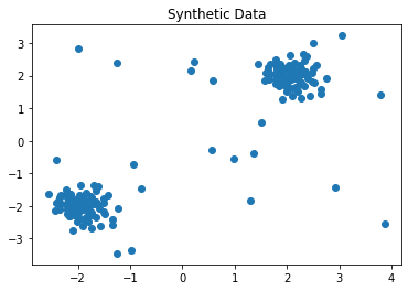
# Fit the model
clf = LocalOutlierFactor(n_neighbors=20, contamination=0.1)
y_pred = clf.fit_predict(X)

# Generate colors based on the prediction
colors = np.array(['#377eb8', '#ff7f00'])
plt.scatter(X[:, 0], X[:, 1], color=colors[(y_pred + 1) // 2])

plt.title("Local Outlier Factor (LOF)")
plt.show()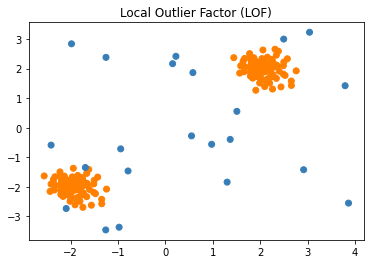
In the above plot, the blue points are the normal data points whereas the orange points are the detected anomalies.
We can now move on to our usual creditcard.csv example:
# Import necessary libraries
import pandas as pd
from sklearn.neighbors import LocalOutlierFactor
from sklearn.preprocessing import StandardScaler
from sklearn.metrics import confusion_matrix

# Load the dataset
data = pd.read_csv('creditcard.csv')

# Set the fraction of data to sample
fraction = 0.1

# We will use stratified sampling to maintain the ratio of anomalies
stratified_data = data.groupby('Class', group_keys=False).apply(lambda x: x.sample(frac=fraction))

# Separate out the features and labels
X_sample = stratified_data.drop('Class', axis=1)
y_sample = stratified_data['Class']

# Standardize the features to have a mean of ~0 and a variance of 1
scaler = StandardScaler()
X_std_sample = scaler.fit_transform(X_sample)

# Train the model
model = LocalOutlierFactor(n_neighbors=20, novelty=True)
model.fit(X_std_sample[y_sample == 0])  # train the model on the normal transactions

# Predict the labels for the entire dataset
y_pred_sample = model.predict(X_std_sample)

# Convert the prediction values to match with 'Class' column in the original dataset
y_pred_sample[y_pred_sample == 1] = 0
y_pred_sample[y_pred_sample == -1] = 1

# Print the confusion matrix
print(confusion_matrix(y_sample, y_pred_sample))
[[27070 1362] [ 5 44]]
Results are:
- True Negatives (27070): The model correctly predicted 27,070 instances where no fraud occurred.
- False Positives (1362): The model incorrectly predicted 1,362 instances of fraud. These are normal transactions that were wrongly flagged as fraudulent.
- False Negatives (5): The model incorrectly predicted 5 instances where fraud occurred but was not flagged. These are fraudulent transactions that went unnoticed by the model.
- True Positives (44): The model correctly flagged 44 instances of fraud.
Overall, the model has done a relatively good job of identifying the fraud cases (44 out of 49), though it has a noticeable number of false positives. The false negatives are very low (5 out of 49 actual fraud cases), indicating the model’s high sensitivity in detecting fraud. This trade-off is often acceptable in fraud detection scenarios, as false negatives (frauds going unnoticed) are typically much more costly than false positives (normal transactions flagged as fraudulent).
However, one should also consider the cost associated with investigating the false positives, as these can also be significant. The choice of model and its parameters should be guided by these considerations.
from sklearn.metrics import classification_report

print(classification_report(y_sample, y_pred_sample))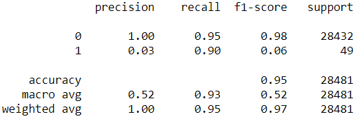
For the “normal” class (0)
- Precision is extremely high, nearly perfect, at 1.00. This means that almost all transactions that the model classified as normal are indeed normal.
- Recall, or the ability of the model to find all the normal transactions, is 0.95, indicating that 95% of the actual normal transactions were correctly identified.
- The F1 score, a combination of precision and recall, is 0.98, which is quite high, showing a good balance of precision and recall.
For the “fraud” class (1)
- Precision is very low, at 0.03. This means that among all transactions that the model classified as fraudulent, only 3% are actually fraudulent. The model has a high false positive rate for fraud transactions.
- Recall, however, is quite high, at 0.90. This indicates that the model was able to correctly identify 90% of the actual fraudulent transactions.
- The F1 score is low, at 0.06, showing an imbalance between precision and recall — recall is high but at the cost of very low precision.
The macro average scores are the unweighted mean values of precision, recall, and F1-score. The weighted average scores are the mean values of precision, recall, and F1-score weighted by the support of each class.
The overall accuracy of the model is 0.95. However, in this case, we should pay more attention to the recall of the fraudulent class, as it is more important to correctly identify as many fraudulent transactions as possible, even at the expense of marking some normal transactions as fraudulent. The high recall score of 0.90 for the fraud class suggests that the model is performing well in this regard.
These results illustrate the challenge of working with imbalanced datasets, and how accuracy can be a misleading metric in these cases. Despite the overall high accuracy, the model’s precision for the fraudulent class is very low, meaning it has many false positives. Nevertheless, the high recall for the fraudulent class indicates it is well-suited to the task of identifying fraudulent transactions, which is the primary goal in this case.
See you in Chapter 10!


