Dealing with Imbalanced Classes in Supervised Learning

A carefully generated, thoroughly engineered resource for Data Scientists.

Part 2 of Chapter 03 from the Guide to Machine Learning for Anomaly Detection

Warning! Before you continue reading this article and all the articles that compose this guide, you must understand this was in part generated using OpenAI’s GPT 4 model. It started as a self learning project and I soon enough realized this could be really valuable to fellow data scientists. Because of this, I will release the entire guide for free alongside every chapter so you can directly go read the guide from the document so you don’t even need to give me reading time if you don’t want to.

Guide Index

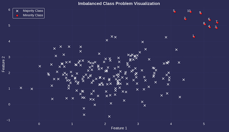
In many real-world classification problems, we are often faced with the situation where the distribution of examples across different classes is not equal — one class may have significantly more examples than the other.

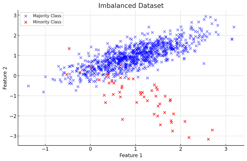
This scenario is known as class imbalance

and the classes are often referred to as the “majority” class (or “negative” class) and the “minority” class (or “positive” class). The terminology of “positive” and “negative” often depends on the problem context; for instance, in a medical diagnosis problem, the “positive” class could be the presence of a disease.

Class imbalance can occur in a variety of domains, such as fraud detection (where fraudulent transactions are usually a tiny fraction of all transactions), email spam detection (where most emails are not spam), or medical diagnosis (where most patients might not have a specific rare disease).

While many machine learning algorithms are designed to work best with balanced class distributions, the reality is that imbalanced classes are quite common, and it’s important to know how to handle them.

An imbalanced dataset can lead to severe issues in model performance, particularly for the minority class.

Machine learning models, particularly the conventional ones, often assume that the classes in a classification problem are balanced.

When the class distribution is severely imbalanced, these models tend to be biased towards the majority class, resulting in poor predictive performance for the minority class.

The impact of this imbalance is that the models end up simply predicting the majority class most of the time, which may lead to very high accuracy but poor recall or precision for the minority class. This happens because the model “learns” that it can maximize overall accuracy (which is often the default metric for model optimization) by always predicting the majority class.

This visualization helps in understanding that when the class distribution is imbalanced, classifiers might be heavily biased towards the majority class, leading to poor predictive performance for the minority class.

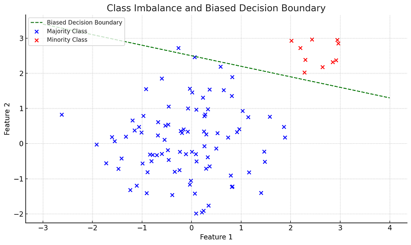
However, in many practical scenarios, the cost of misclassifying the minority class instances can be much higher. For example, in a fraud detection problem, failing to identify a fraudulent transaction (a case of the minority class) could have much more serious consequences than misclassifying a non-fraudulent transaction.

Hence, the class imbalance problem poses a challenge for the predictive performance of machine learning models, especially for those applications where the minority class is of great interest. In the following sections, we will explore various methods to address this issue.

Strategies for Dealing with Imbalanced Classes

There are several strategies to handle imbalanced classes. Each strategy has its strengths and weaknesses, and the choice of strategy should depend on the specific context of the problem. Here, we discuss three primary strategies:

Resampling Techniques

This involves adjusting the class distribution in the training data. There are two main types of resampling:

Oversampling: This involves increasing the number of minority class instances. One popular method is Synthetic Minority Over-sampling Technique (SMOTE), which creates synthetic instances of the minority class. However, oversampling can lead to overfitting if the synthetic instances are too similar to the existing ones.

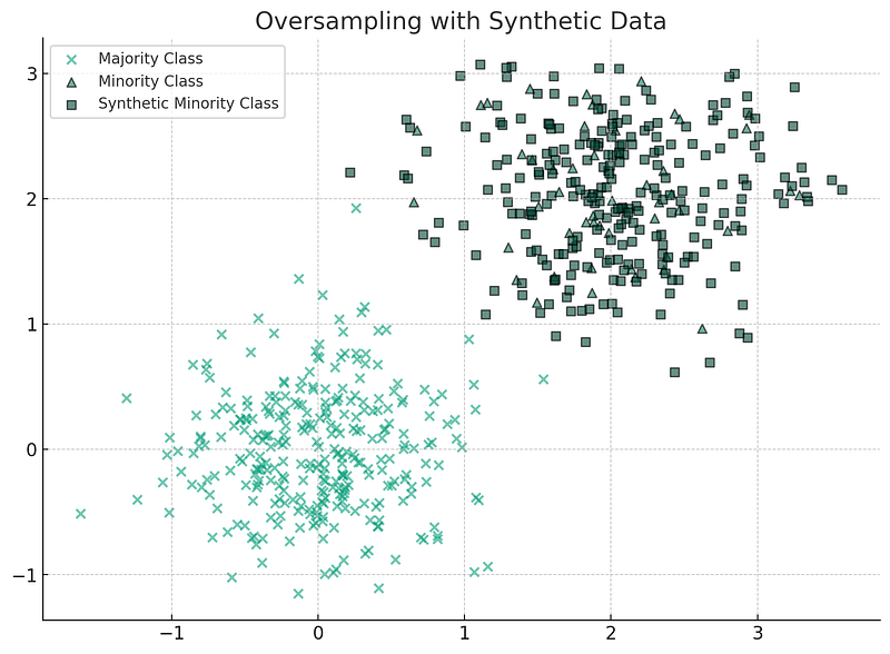
Undersampling: This involves reducing the number of majority class instances. While this can help balance the classes, it also results in loss of data, which could be problematic if the original dataset is not large enough.

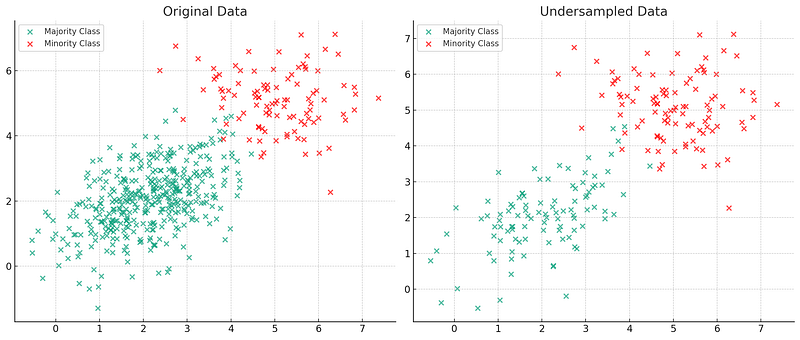
Cost-Sensitive Training

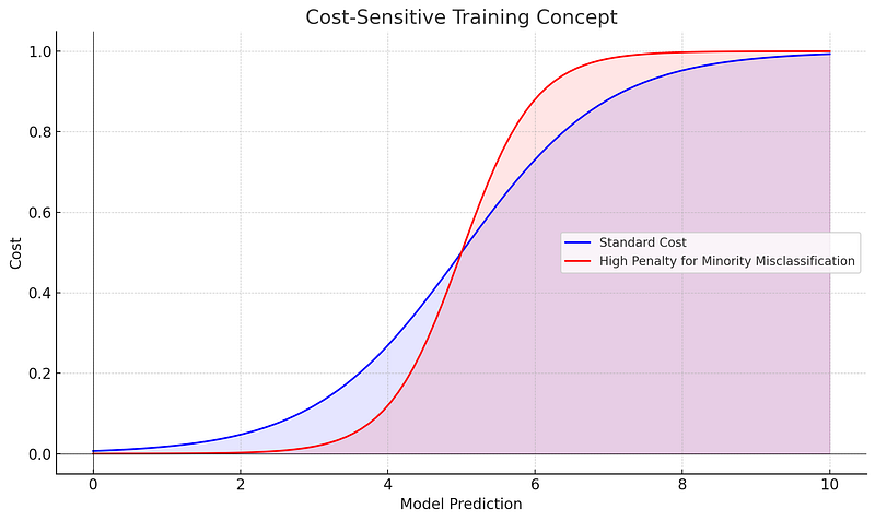
This involves adjusting the cost function used in training the model, such that misclassifying the minority class instances incurs a higher penalty. This strategy does not involve changing the training data, and it can be a powerful method when combined with the right model.

Ensemble Methods

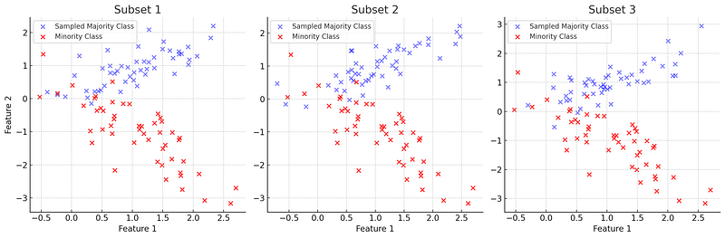
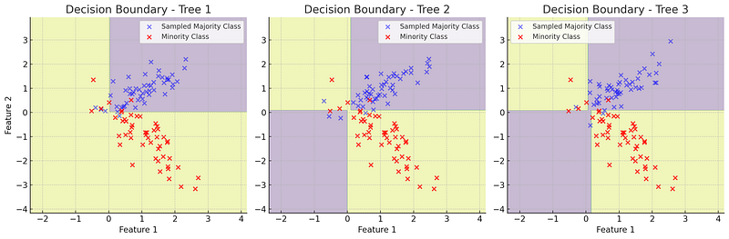
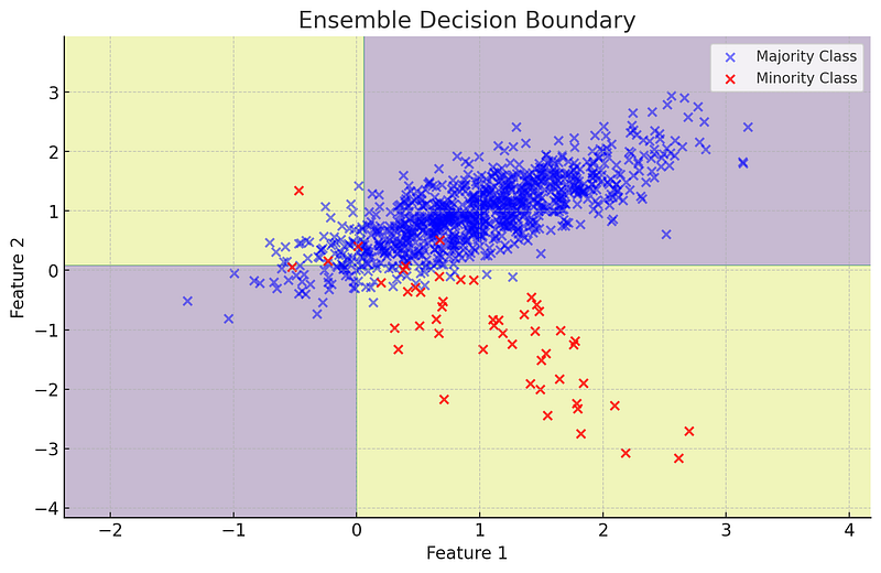
This involves combining multiple machine learning models to improve the prediction of the minority class. For instance, one can use undersampling in conjunction with bagging (Bootstrap Aggregating) to create an ensemble of models, each trained on a different subset of the majority class instances. This strategy, known as Balanced Random Forests, can significantly improve the prediction of the minority class.

As we can see, the minority class is vastly outnumbered by the majority class.

Here are three subsets created through the process of undersampling

Here we have the decision boundaries for each tree, trained on its respective subset

This visualization shows the power of ensemble methods. By training multiple models on different subsets and then combining their predictions, we can achieve a more robust and comprehensive decision boundary that can better generalize and capture the minority class.

Evaluation Metrics for Imbalanced Classes

In problems with imbalanced classes, using accuracy as the evaluation metric can be misleading. For instance, if we have a dataset where 99% of the instances are of the majority class, a model that simply predicts the majority class for every instance will have an accuracy of 99%, even though it completely fails to identify the minority class.

To overcome this, we use the metrics that give us more information about how well the model is doing on each class, which we have seen in previous chapters:

Precision

Precision is the proportion of true positive predictions (i.e., instances correctly identified as belonging to the positive class) out of all positive predictions made. A higher precision means fewer false positives (i.e., instances incorrectly identified as belonging to the positive class).

Recall (or Sensitivity)

Recall is the proportion of true positive predictions out of all actual positive instances. A higher recall means fewer false negatives (i.e., positive instances that were incorrectly identified as negative).

F1 Score

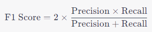
The F1 Score is the harmonic mean of precision and recall. It provides a single score that balances both precision and recall. A higher F1 Score means better model.

Area Under the Receiver Operating Characteristic Curve (AUC-ROC)

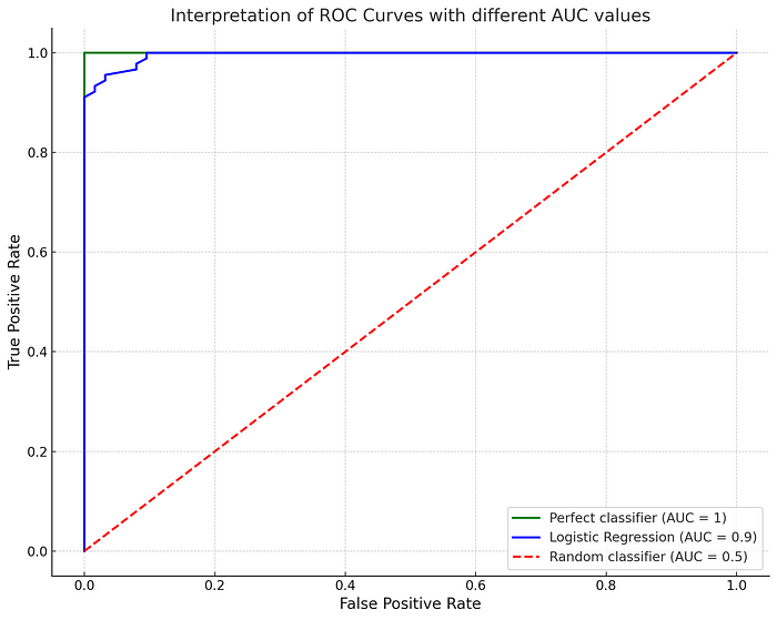
The ROC curve is a plot of the true positive rate (recall) against the false positive rate (1-specificity) for various threshold values. The AUC is the area under the ROC curve, and it represents a model’s ability to correctly classify instances across all threshold values. An AUC of 0.5 suggests no discrimination (i.e., the model is no better than random guessing), while an AUC of 1.0 suggests perfect discrimination.

Confusion Matrix

A confusion matrix is a table that describes the performance of a classification model. It presents the true positives, true negatives, false positives and false negatives, providing a comprehensive overview of the model performance.

Coding Time: Application of Techniques for Imbalanced Classes on Real Dataset

In this section, we will demonstrate the application of various techniques to handle imbalanced classes, using a real-world dataset. We will be using the “Credit Card Fraud Detection” dataset from Kaggle, which is highly imbalanced. It consists of transactions made by credit cards, where the positive class (frauds) account for only 0.172% of all transactions.

To follow along with this case study, you will need to download the dataset from Kaggle. You can find it in the code repo in Github or here: https://www.kaggle.com/datasets/arockiaselciaa/creditcardcsv?select=creditcard.csv

Download the creditcard.csv file and save it in the same directory as your python script.

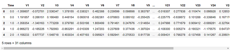
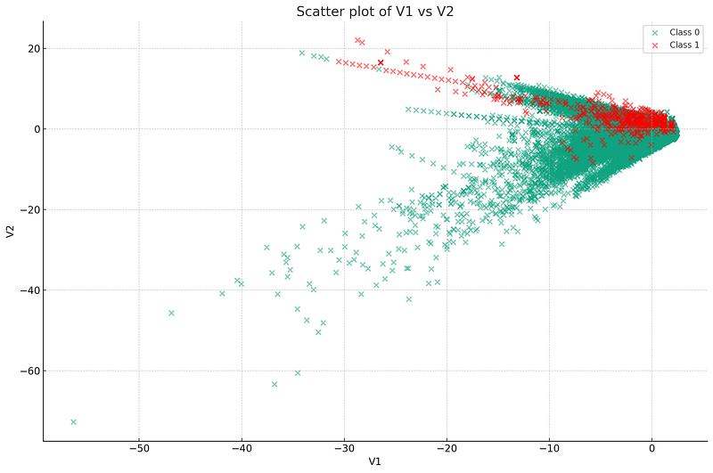
The dataset contains only numerical input variables which are the result of a PCA transformation. Unfortunately, due to confidentiality issues, we do not have the original features and more background information about the data. Features V1, V2, … V28 are the principal components obtained with PCA, the only features which have not been transformed with PCA are ‘Time’ and ‘Amount’. ‘Time’ contains the seconds elapsed between each transaction and the first transaction in the dataset. The feature ‘Amount’ is the transaction Amount, this feature can be used for example-dependant cost-sensitive learning. Feature ‘Class’ is the response variable and it takes value 1 in case of fraud and 0 otherwise.

Let’s apply the techniques discussed in the previous sections to this dataset. We will first load the dataset and perform an exploratory data analysis. Then, we will split the data into training and testing sets and build a model using the original, imbalanced dataset. Following that, we will apply various techniques to handle the imbalanced classes and compare the performance of the models trained on the balanced datasets.

Please note that due to the complexity of this case study and the limitations of the dataset, the results might not be perfect or applicable to all scenarios. The purpose of this case study is to demonstrate how to apply these techniques, rather than providing a definitive solution to credit card fraud detection. Always make sure to understand the data and the problem at hand before deciding on the best approach.

# Import necessary libraries
import pandas as pd
from sklearn.model_selection import train_test_split
from sklearn.linear_model import LogisticRegression
from sklearn.metrics import confusion_matrix, classification_report

# Load the dataset
df = pd.read_csv('creditcard.csv')

# Print the first 5 rows of the dataframe.
df.head()

# Print the distribution of 'Class' variable
print('\nClass Distribution:')
print(df['Class'].value_counts())

Class Distribution: Class 0: 284315 Class 1: 492

# Divide the data into features (X) and target variable (y)
X = df.drop('Class', axis=1)
y = df['Class']

# Split the data into training and testing sets
X_train, X_test, y_train, y_test = train_test_split(X, y, test_size=0.2, random_state=42)

# Initialize the Logistic Regression model
model = LogisticRegression()

# Fit the model
model.fit(X_train, y_train)

# Make predictions
y_pred = model.predict(X_test)

# Print the confusion matrix
print('\nConfusion Matrix:')
print(confusion_matrix(y_test, y_pred))

With this code we begin with a simple benchmarking approach were we just fit a logistic regression model to our imbalanced data without any treatment.

Confusion Matrix: [[56829 35] [ 41 57]]

# Print the classification report
print('\nClassification Report:')
print(classification_report(y_test, y_pred))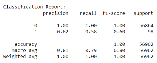

The classification report shows that the model is nearly perfect (accuracy of 1.00) when predicting the majority class (0) but struggles to correctly predict the minority class (1). This is evidenced by the low precision (0.62) and recall (0.58) for the minority class. In other words, when the model predicts that a transaction is fraudulent (class 1), it’s correct only about 62% of the time. Furthermore, it’s only identifying 58% of the total fraudulent transactions in the dataset.

This is not surprising given the highly imbalanced nature of the dataset, and it illustrates why accuracy (99%) is not a reliable metric in this context. The high accuracy is driven by the large number of true negatives (legitimate transactions correctly identified as such), while the relatively small number of fraud cases (class 1) significantly impact precision and recall, but not accuracy. The F1 score, which balances precision and recall, is also quite low at 0.60 for the minority class. This tells us that we need to improve our model’s ability to detect the minority class (fraudulent transactions).

Now, let’s proceed with implementing the first technique to handle imbalanced classes:

Undersampling

Under-sampling balances the dataset by reducing the size of the abundant class. This method is used when quantity of data is sufficient. By keeping all samples in the rare class and randomly selecting an equal number of samples in the abundant class, a balanced new dataset can be retrieved for further modelling.

from sklearn.linear_model import LogisticRegression
from imblearn.under_sampling import RandomUnderSampler

# initialize the undersampler
rus = RandomUnderSampler(random_state=0)

# fit the sampler to the data
X_under, y_under = rus.fit_resample(X_train, y_train)

Now we can see how undersampling balanced our classes. While before we had:

y_train.value_counts()

Class 0: 227451 Class 1: 394

Now we have:

y_under.value_counts()

Class 0: 394 Class 1: 394

# now let's fit the Logistic Regression model on this undersampled data
lr = LogisticRegression(random_state=0)
lr.fit(X_under, y_under)

# make predictions
y_pred = lr.predict(X_test)

# Print the confusion matrix
print('\nConfusion Matrix:')
print(confusion_matrix(y_test, y_pred))

Confusion Matrix: [[54948 1916] [ 8 90]]

# print classification report
print(classification_report(y_test, y_pred))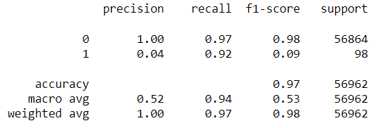

The classification report of the Logistic Regression model trained with the RandomUnderSampling technique reveals interesting results. The model’s recall score for the minority class (fraudulent transactions) has significantly improved, reaching 0.92. This means that the model is able to correctly identify 92% of the actual fraudulent transactions, which is a significant improvement over the initial model that was not trained with under-sampling.

However, this has come at the cost of a decreased precision for the minority class, which has dropped to 0.04. This low precision score indicates that among all the transactions that the model has predicted to be fraudulent, only 4% of them are actually fraudulent. This means that the model is producing a significant number of false positives.

The decrease in precision has led to a very low f1-score for the minority class, which is 0.09. The f1-score considers both precision and recall, providing a balanced measure of the model’s performance, and this low score indicates that while the model is identifying the fraudulent transactions better (high recall), it is also incorrectly flagging many legitimate transactions as fraudulent (low precision).

On the other hand, for the majority class (legitimate transactions), the precision is still very high (1.00) but the recall has slightly decreased to 0.97.

The accuracy of the model, considering both classes, has also slightly decreased to 0.97.

In summary, the use of under-sampling has helped to improve the model’s ability to identify fraudulent transactions but it has also increased the number of false positives, leading to more legitimate transactions being incorrectly flagged as fraudulent.

This could be problematic in a real-world setting as it could lead to customer dissatisfaction. Therefore, when using under-sampling, it’s crucial to consider the trade-off between detecting more actual fraudulent transactions (increasing recall) and not flagging too many legitimate transactions as fraudulent (maintaining a reasonable precision).

Oversampling

The next technique that we are going to explore is Oversampling, specifically Synthetic Minority Over-sampling Technique (SMOTE). Oversampling techniques aim to balance the class distribution by increasing the size of rare samples. Instead of getting rid of abundant samples, new rare samples are generated to get a balanced dataset.

SMOTE is an oversampling technique where the synthetic samples are generated for the minority class.

This algorithm helps to overcome the overfitting problem posed by random oversampling. It focuses on the feature space to generate new instances with the help of interpolation between the positive instances that lie together.

Let’s implement this technique using the same credit card fraud dataset and evaluate its impact on our Logistic Regression model’s performance.

# Install the necessary library
# !pip install imbalanced-learn

# Import the necessary libraries
from imblearn.over_sampling import SMOTE

# Apply SMOTE technique
smote = SMOTE(random_state=42)
X_train_smote, y_train_smote = smote.fit_resample(X_train, y_train)

y_train.value_counts()

Class 0: 227451 Class 1: 394

Now we can see our classes are balanced:

y_train_smote.value_counts()

Class 0: 227451 Class 1: 227451

# Train Logistic Regression model
model = LogisticRegression(random_state=0)
model.fit(X_train_smote, y_train_smote)

# Make predictions
y_pred = model.predict(X_test)

# Print the confusion matrix
print('\nConfusion Matrix:')
print(confusion_matrix(y_test, y_pred))

Confusion Matrix: [[55885 979] [ 11 87]]

# Print the classification report
print(classification_report(y_test, y_pred))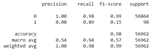

The classification report for the model trained with oversampling technique (SMOTE) shows some promising results.

As a reminder, precision is the number of true positive results divided by the number of all positive results (including those not identified correctly), and recall is the number of true positive results divided by the number of all samples that should have been identified as positive.

From the report, we can see that for class 0 (non-fraud transactions), the precision is still very high (1.00), indicating that when the model predicts a transaction is non-fraud, it is almost always correct. The recall, which is also 0.98, indicates that the model has correctly identified 98% of all actual non-fraud transactions.

For class 1 (fraud transactions), the precision is lower at 0.08, suggesting that the model incorrectly marks a number of non-fraud transactions as fraud. However, the recall of 0.89 shows a strong improvement over the original model. This means that the model correctly identifies 89% of all actual fraud transactions, even though it does produce some false positives (non-fraud transactions incorrectly identified as fraud).

The F1-score for the fraud class has also improved significantly compared to the previous models. This score is the harmonic mean of precision and recall, and it tries to balance these two measures. An improved F1-score suggests a better overall performance of the model for the fraud class.

The overall accuracy of the model is 0.98, which suggests that the model is doing a good job of identifying both fraud and non-fraud transactions. However, as we discussed earlier, accuracy might not be the best metric to evaluate the performance for imbalanced classes.

In conclusion, by using SMOTE, we’ve made the model much better at identifying fraud transactions (higher recall) at the expense of introducing more false positives (lower precision for class 1).

In many practical scenarios, it may be considered acceptable to have a few more false positives, as long as we are able to catch a higher proportion of the fraud cases. The appropriate balance will depend on the specific costs associated with false positives and false negatives.

Synthetic Minority Over-sampling Technique combined with Edited Nearest Neighbours (SMOTEENN)

The third method we will explore in this chapter is the SMOTEENN technique, which combines over-sampling and under-sampling techniques. Specifically, it uses SMOTE (Synthetic Minority Over-sampling Technique) for over-sampling and Edited Nearest Neighbours (ENN) for under-sampling.

The SMOTE technique works by selecting instances that are close in the feature space, drawing a line between the instances in the feature space, and drawing a new sample at a point along that line. On the other hand, ENN removes any instance whose class label differs from the class of at least half of its k nearest neighbors.

As a combination of over and under-sampling, SMOTEENN can help balance the dataset effectively.

However, note that SMOTEENN is computationally more expensive as it involves the generation of synthetic examples and cleaning the majority class.

Here’s an illustration of the entire process:

Original Imbalanced Dataset: The initial dataset with a clear imbalance between Class #0 (blue) and Class #1 (red).
Dataset after Manual SMOTE: After applying SMOTE, synthetic samples (cyan) are added to the minority class (Class #0). These synthetic samples are positioned between the original instances of the minority class.
Dataset after SMOTEENN: After applying ENN, some of the majority class samples (Class #1) that were deemed as noise or borderline are removed, leading to a more balanced dataset.

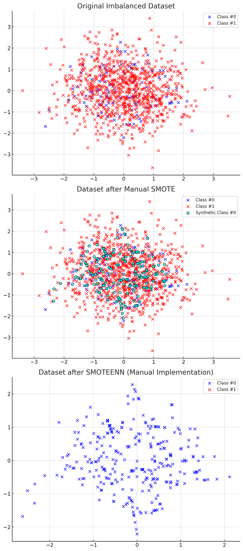
Let’s apply the SMOTEENN technique to our data:

from imblearn.combine import SMOTEENN

# Implementing the SMOTEENN technique
smote_enn = SMOTEENN(random_state=0)
X_resampled, y_resampled = smote_enn.fit_resample(X, y)

# Train and fit the logistic regression model on the resampled data
model_resampled = LogisticRegression(max_iter=1000)
model_resampled.fit(X_resampled, y_resampled)

# Make predictions and evaluate the model
y_pred_resampled = model_resampled.predict(X_test)

print('Classification Report:')
print(classification_report(y_test, y_pred_resampled))

This piece of code first applies the SMOTEENN technique to the training data. Then it trains a logistic regression model on the resampled data and uses it to make predictions on the test data. The results are displayed in the form of a classification report.

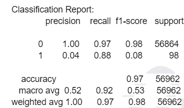
Note: The above code might take longer to run than the previous ones due to the computationally intensive nature of SMOTEENN.

When we compare the SMOTEENN, undersampling and oversampling results, we notice that they all make significant improvements in terms of identifying the minority class (Class 1: Fraudulent transactions) compared to the original model. However, the key differences are seen in the precision and recall values for the minority class, and the overall accuracy.

In the case of undersampling

The model had a precision of 0.04 and recall of 0.92 for the minority class. This indicates that while the model was able to correctly identify 92% of the fraudulent transactions, it also incorrectly classified a significant number of non-fraudulent transactions as fraudulent, which is reflected in the low precision.

In the case of oversampling

The model had a precision of 0.08 and a recall of 0.89 for the minority class. While the precision here is better than that of the undersampling method, it is still low indicating a high number of false positives. However, the model correctly identifies 89% of the fraudulent transactions which is still high.

Finally, in the case of SMOTEENN

The model has a precision of 0.04 and a recall of 0.88 for the minority class, showing similar results to the undersampling model.

In all cases, the precision for the majority class remains at 1.00 indicating that almost all transactions identified as non-fraudulent were indeed so.

In conclusion, all three techniques improved the detection of fraudulent transactions compared to the original model. However, this comes with the cost of increasing the number of false positives, as seen in the low precision scores for the minority class.

Depending on the specific business case and the cost associated with false positives and false negatives, one method might be preferable over the others.

Cost-Sensitive Training

In many real-world classification problems, misclassification costs are different for different classes. This is certainly true for our fraud detection problem where incorrectly identifying a fraudulent transaction (false negative) may cost the company a significant amount of money, whereas falsely identifying a legitimate transaction as fraudulent (false positive) might cause inconvenience to the customer but won’t necessarily have a significant monetary cost.

Cost-sensitive training is a method in which the misclassification costs are incorporated directly into the training process. This method aims to minimize the total misclassification cost rather than the number of misclassification errors.

In our case, we can assign a high cost to misclassifying a fraudulent transaction and a lower cost to misclassifying a legitimate transaction.

C(TP): would be the cost when a transaction is fraudulent and the system correctly identifies it as fraudulent. Typically, this cost is 0 because it’s a correct classification. C(FN): would be the cost when a transaction is fraudulent but the system fails to identify it. This cost is high because the fraudulent transaction goes undetected, potentially leading to significant financial losses. C(FP): would be the cost when a transaction is legitimate, but the system incorrectly identifies it as fraudulent. This might inconvenience the customer, and may also involve some operational costs for the company to resolve the issue. However, it’s typically much lower than the cost of a false negative. C(TN): would be the cost when a transaction is legitimate and the system correctly identifies it as such. Like $C(TP)$, this cost is typically 0 because it’s a correct classification.

Given the above, let’s assume: C(FN) = $1000: Cost of missing a fraudulent transaction. C(FP) = $50: Cost of falsely flagging a legitimate transaction.

Using these values, our cost matrix for the fraud detection scenario will look something like this:

This matrix clearly illustrates the disparity in costs between falsely flagging a legitimate transaction and missing a fraudulent one. It’s a powerful tool to communicate the cost implications of different types of classification errors to stakeholders.

Several machine learning algorithms, such as Decision Trees, Random Forests, and Support Vector Machines, have provisions for including these costs in their training process.

To apply cost-sensitive training, we need to modify our model fitting code to include the class_weight parameter. This is a dictionary that receives as keys the classes and as values the weight that we want to assign to each misclassification.

Let’s see how this technique would affect our logistic regression model.

from sklearn.linear_model import LogisticRegression

# Define the weights
weights = {0:1, 1:10}

# Instantiate the Logistic Regression model with cost-sensitive training
model = LogisticRegression(class_weight=weights)

# Fit the model
model.fit(X_train, y_train)

# Predict on the test set
y_pred = model.predict(X_test)

# Print the classification report
print(classification_report(y_test, y_pred))

# Print the confusion matrix
print('\nConfusion Matrix:')
print(confusion_matrix(y_test, y_pred))

This code will apply a higher cost to misclassifying fraudulent transactions by setting the weight for class 1 to 10 and class 0 to 1.

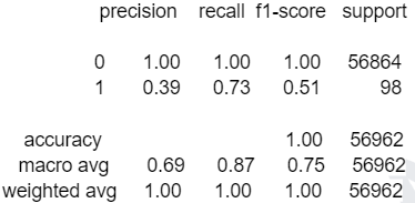
Confusion Matrix: [[56750 114] [ 26 72]]

In the cost-sensitive model, we see a shift in the metrics compared to the original logistic regression model. Specifically, the recall of the minority class (fraudulent transactions) has increased from 0.58 to 0.73. This improvement indicates that the cost-sensitive model is better at identifying fraudulent transactions than the original model.

On the other hand, the precision for the minority class has dropped from 0.62 to 0.39. This decrease in precision indicates that while our model is catching more of the fraudulent transactions, it is also incorrectly identifying more legitimate transactions as fraudulent.

This shift is expected and is an illustration of the precision-recall trade-off: as our model becomes more aggressive in predicting fraudulent transactions (thereby increasing recall), it also ends up misclassifying more legitimate transactions as fraudulent (thereby decreasing precision).

However,

the high recall rate may be desirable in our case because missing a fraudulent transaction could be much costlier than a false alarm.

In conclusion, using cost-sensitive training has allowed us to improve the model’s ability to catch fraudulent transactions, albeit at the cost of more false positives. The choice of whether this trade-off is acceptable will depend on the specific costs associated with false negatives (missed fraudulent transactions) and false positives (legitimate transactions incorrectly flagged as fraudulent).

Ensemble Methods — Balanced Random Forest

Ensemble methods combine the decisions from multiple machine learning models to improve overall performance.

It is like getting second opinions from different doctors before proceeding with a major operation — the decision is typically more reliable when it is consensus-based.

When dealing with imbalanced data, ensemble methods can be particularly useful. For example, we can combine undersampling of the majority class with bagging to create a method known as the Balanced Random Forest (BRF).

In BRF, each tree in the forest is built on a different subset of majority class instances, combined with all instances of the minority class.

The combination of different ‘views’ on the majority class helps to better identify the distinguishing features of the minority class, hence improving its prediction.

As in the previous sections, we’ll use the credit card fraud dataset for this example. We will use the BalancedRandomForestClassifier from the imblearn library.

from imblearn.ensemble import BalancedRandomForestClassifier
from sklearn.metrics import classification_report

# Create an instance of the classifier
brf = BalancedRandomForestClassifier(n_estimators=100, random_state=0)

# Train the classifier
brf.fit(X_train, y_train)

# Make predictions on the test set
y_pred = brf.predict(X_test)

# Print the classification report
print("Classification Report: \n", classification_report(y_test, y_pred))

# Print the confusion matrix
print('\nConfusion Matrix:')
print(confusion_matrix(y_test, y_pred))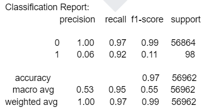

Confusion Matrix: [[55403 1461] [ 8 90]]

Looking at the classification report for the Balanced Random Forest model, we observe that the precision for the minority class (1) is 0.06, recall is 0.92, and the f1-score is 0.11. The precision is low, meaning that the model predicts quite a few false positives. However, the recall is high, which suggests that the model is able to correctly identify most of the actual instances of the minority class. The f1-score, which balances precision and recall, is fairly low due to the low precision.

When comparing to our other techniques, the Balanced Random Forest model outperforms all other techniques in terms of recall, i.e., its ability to find all the positive instances. This is a significant advantage when the cost of false negatives is high. For example, in fraud detection, it is generally more acceptable to have false alarms (false positives) than to miss a fraudulent transaction (false negatives).

The precision of this method is not as high as that of the original Logistic Regression or the Cost-Sensitive Training model, which suggests that this method might lead to a higher number of false positives. Whether this trade-off is acceptable depends on the specific cost associated with false positives in the given context.

Finally, it’s important to remember that these results may vary with different random state settings or when applied to different datasets. It is recommended to always try multiple methods and select the one that best meets your specific requirements and constraints.

Why Balanced Random Forest and not plain Random Forest?

A Balanced Random Forest (BRF) is a variation of the traditional Random Forest algorithm that is designed to handle imbalanced datasets more effectively.

The Random Forest algorithm constructs a multitude of decision trees at training time and outputs the mode of the classes (classification) or mean prediction (regression) of the individual trees. It is a powerful machine learning method that often performs very well right out of the box. However, like many other machine learning methods, it can be less effective when dealing with highly imbalanced datasets. That’s because the algorithm can be biased towards the majority class, and hence may not perform well on the minority class.

On the other hand,

the Balanced Random Forest algorithm addresses this issue by changing the underlying dataset for each tree in the forest. It does so by undersampling the majority class, i.e., randomly removing some samples from the majority class to balance the class distribution.

This process ensures that the model sees an approximately equal number of instances from each class, which helps to alleviate the problem of the model being biased towards the majority class.

As a result, Balanced Random Forests tend to offer better performance than traditional Random Forests when dealing with imbalanced datasets. They are often more successful at correctly classifying instances from the minority class.

It’s important to note that these models have different strengths and weaknesses. While Balanced Random Forests can be better at handling imbalanced data, they may not always be the best choice depending on the specific data and problem at hand. It’s always a good idea to try different approaches and evaluate their performance to find the best model for your specific needs.

See you in chapter 5!

Link to Chapter 4 code: https://github.com/gabrielpierobon/anomaly_detection/blob/main/Chapter%2004%20Dealing%20with%20Imbalanced%20Classes%20in%20Supervised%20Learning.ipynb

Link to PDF Guide: https://drive.google.com/file/d/1g77lB2zeZGQUqIyPSb9Fr-uMyjmAG4j4/view?usp=drive_link