K-Means Clustering for Anomaly detection

A carefully generated, thoroughly engineered resource for Data Scientists.

Chapter 05 from the Guide to Machine Learning for Anomaly Detection

Warning! Before you continue reading this article and all the articles that compose this guide, you must understand this was in part generated using OpenAI’s GPT 4 model. It started as a self learning project and I soon enough realized this could be really valuable to fellow data scientists. Because of this, I will release the entire guide for free alongside every chapter so you can directly go read the guide from the document so you don’t even need to give me reading time if you don’t want to.

Guide Index

Our exploration of machine learning thus far has largely focused on supervised learning, a realm where models are trained on labeled data to predict outcomes or classify data points.

While supervised learning offers a powerful toolset for a wide array of applications, it requires a significant amount of labelled data, which might be difficult, time-consuming or costly to obtain.

Moreover, it is more reactive than proactive in that it responds to what it has seen during training.

On the other hand, unsupervised learning, the focus of this chapter, offers an alternative approach where models are trained to infer patterns from data without prior labels or classification. Here,

the algorithms uncover hidden structures within the data, working to understand the underlying distributions or to find relationships among variables.

This is a powerful mechanism, particularly for tasks where we are unsure of what to look for or when dealing with novel data where predefined labels may not exist or are insufficient.

A salient application of unsupervised learning is anomaly detection. In a vast ocean of data, anomalies are like tiny islands that deviate from the mainland.

These anomalies can be indicators of critical incidents such as credit card fraud, network intrusion, or equipment failure. As these anomalies represent unforeseen events, we do not always have pre-labeled examples to train a supervised learning model. This is where unsupervised learning, with its power to detect and delineate patterns and structures without explicit guidance, comes to the fore.

Anomaly detection, in the context of machine learning, is about identifying data points or patterns that deviate significantly from the norm.

These could be outliers, novelties, noise, or exceptions, all of which hold potential insights. Anomaly detection can be of immense value across a broad array of industries, from finance to healthcare, IT to manufacturing, and beyond.

One of the widely used techniques for anomaly detection within the realm of unsupervised learning is K-Means Clustering.

It is a simple yet powerful algorithm that groups data points into clusters based on their feature similarity. As we progress through this chapter, we’ll introduce the K-Means Clustering algorithm and showcase its utility in anomaly detection using a real-world dataset.

Understanding the K-Means Clustering Algorithm

Before we delve into how K-Means aids in anomaly detection, it’s crucial to understand how the algorithm works.

K-Means is a partitioning-based clustering algorithm, a type of unsupervised learning method that organizes unlabeled data into groups based on their inherent patterns or similarities. The ‘K’ in K-Means refers to the number of clusters that the algorithm will identify in the data, which is specified a priori.

We can make up some data to introduce the topic:

import matplotlib.pyplot as plt
from sklearn.datasets import make_blobs

# Generate sample data
X, y = make_blobs(n_samples=300, centers=2, cluster_std=0.80, random_state=0)

# Plot the data points
plt.scatter(X[:, 0], X[:, 1])

plt.title('Unlabeled Data')
plt.show()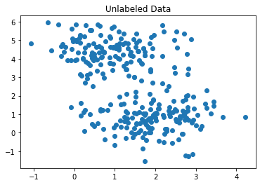

The K-Means Algorithm

The operation of K-Means involves the following iterative steps:

Initialization: Randomly select ‘K’ data points from the dataset. These points act as the initial centroids for the clusters.

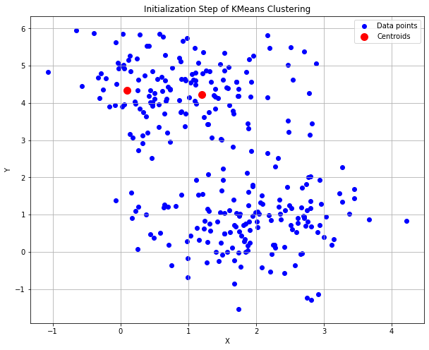
2. Assignment: Assign each data point in the dataset to the nearest centroid, forming K clusters. The measure of nearness is typically Euclidean distance, although other distance measures can also be used.

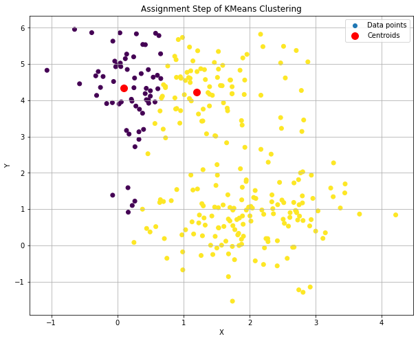
3. Update: For each of the K clusters, compute the new centroid as the mean of all the data points assigned to that cluster.

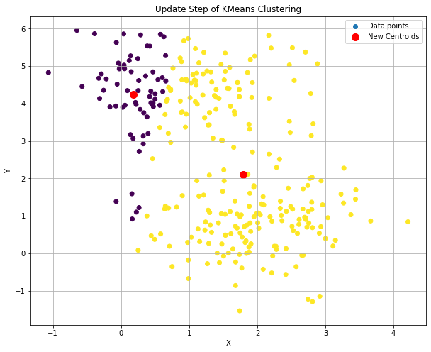
4. Repeat: Repeat steps 2 and 3 until a stopping criterion is met. This could be a set number of iterations, or when the assignment of data points to clusters no longer changes (i.e., the algorithm has converged).

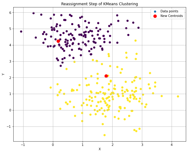
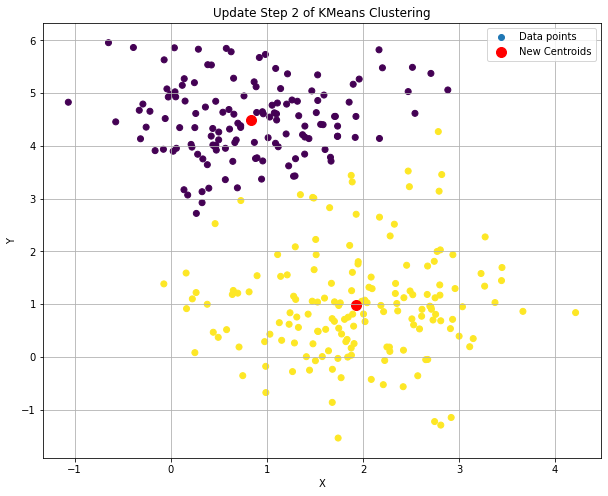
(this process continues until no assignment changes…)

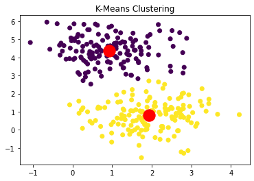
At the end of this process, we have K clusters, each represented by its centroid. Each data point belongs to the cluster with the closest centroid.

Coding Time: Using the KMeans algorithm

Let’s solve the last example in a few lines of code…

import matplotlib.pyplot as plt
from sklearn.datasets import make_blobs
from sklearn.cluster import KMeans

# Generate sample data
X, y = make_blobs(n_samples=300, centers=2, cluster_std=0.8, random_state=0)

# Run K-Means
kmeans = KMeans(n_clusters=2)
kmeans.fit(X)

# Plot the data points
plt.scatter(X[:, 0], X[:, 1], c=kmeans.labels_, cmap='viridis')

# Plot the centroids
plt.scatter(kmeans.cluster_centers_[:, 0], kmeans.cluster_centers_[:, 1], s=300, c='red')

plt.title('K-Means Clustering')
plt.show()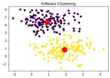

Preprocessing and Feature Selection for K-Means

Preprocessing data for K-Means involves several key steps that are important to achieving accurate results. The process of transforming raw data into an understandable format is crucial since the quality of data and the useful information that can be derived from it directly affects the ability of our model to learn effectively.

Scaling

One of the first preprocessing steps is scaling.

Since K-Means clustering is a distance-based algorithm, the range of values in each feature can have a direct impact on the result.

For instance, a feature that ranges from 0 to 1000 will overshadow a feature that only ranges from 0 to 1, and will have a larger influence on the distance computation, potentially leading to a bias towards the feature with larger values.

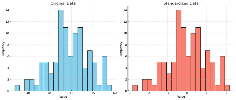
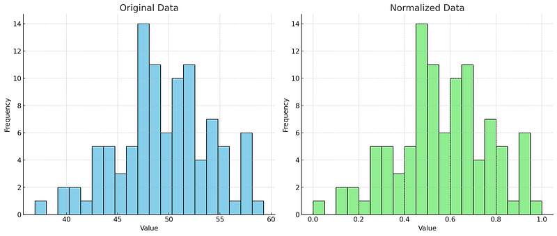
Therefore, it’s usually a good idea to scale the data so that all features have similar ranges. Two common scaling methods are standardization and normalization.

Standardization transforms the data to have zero mean and unit variance

On the left, we have the Original Data which is distributed around a mean that is not 0, and with a standard deviation that is not 1. On the right, after standardization, the Standardized Data has a mean of 0 and a standard deviation of 1.

Normalization scales the data to fall within a smaller, specific range, such as 0 to 1.

On the left, we again have the Original Data. On the right, the Normalized Data has been scaled to lie between 0 and 1.

Handling Categorical Variables

Another important preprocessing step for K-Means is dealing with categorical variables. The K-Means algorithm calculates distances between data points to form clusters, and the concept of distance is not directly applicable to categorical variables.

There are several strategies for dealing with categorical data, including:

1. One-Hot Encoding: This technique converts a categorical variable with n categories into n binary features, with only one active feature for each data point. This method is effective but can lead to a large increase in dataset size if a categorical variable has many categories.

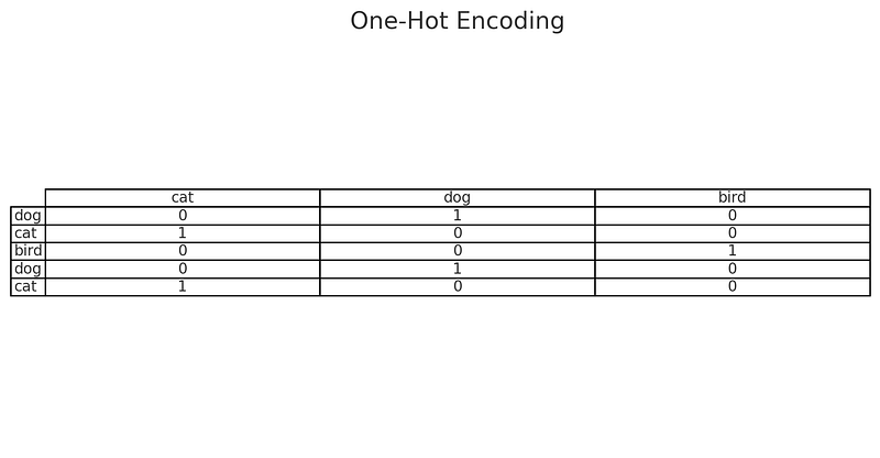
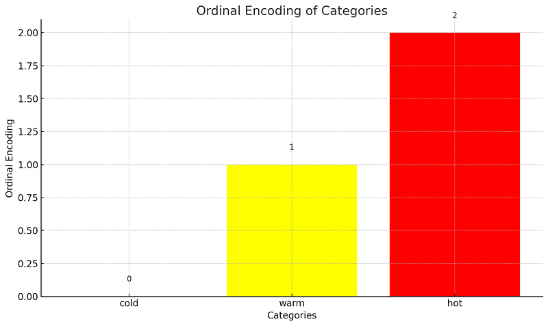
For instance, the data point “dog” is encoded as `[0, 1, 0]`, indicating that it corresponds to the "dog" category. Similarly, "cat" is encoded as `[1, 0, 0]`.

2. Ordinal Encoding: This technique converts categorical variables into numerical values. It’s useful when the categorical variable has a natural ordered relationship (like ‘cold’, ‘warm’, ‘hot’).

The categorical variables, such as ‘cold’, ‘warm’, and ‘hot’, are represented on the x-axis. Their corresponding ordinal encodings, namely 0, 1, and 2, are displayed on the y-axis. The bar colors (blue for ‘cold’, yellow for ‘warm’, and red for ‘hot’) further emphasize the increasing order or intensity of the categories.

3. Binary Encoding: This technique first encodes the categories into ordinal numbers, and then these numbers are converted into binary code. This results in fewer new features compared to one-hot encoding.

Note that each method has its own strengths and weaknesses, and the choice of method often depends on the specific dataset and the business context.

Feature Selection for K-Means

Feature selection is an important step when we have a large number of features.

It involves selecting the most useful features to train our model.

Reducing the dimensionality of the dataset can make the K-Means algorithm faster and more effective, as it reduces noise and irrelevant details. This can be especially beneficial in high-dimensional data where irrelevant features might distract the model from learning the underlying patterns.

There are various methods for feature selection, such as:

1. Filter Methods: These are often used as a preprocessing step. These methods include linear correlation, chi-square test, information gain, and others.

2. Wrapper Methods: These consider the selection of a set of features as a search problem, where different combinations are prepared, evaluated and compared with other combinations. Methods include recursive feature elimination, genetic algorithms, and others.

3. Embedded Methods: These methods learn the best set of features during the model training process. Methods include LASSO, Elastic Net, Ridge Regression, and others.

Choosing which features to keep or discard will also require domain knowledge, as well as experimentation.

After preprocessing and feature selection, our data will be ready for applying the K-Means algorithm. In the next sections, we’ll discuss how to implement and apply K-Means for anomaly detection.

Coding Time: Detecting credit card fraud with K-Means

Our objective is to use K-Means clustering for anomaly detection in the “creditcard.csv” dataset from Kaggle, which contains transactions made by European credit cardholders. We will preprocess the data, perform K-Means clustering, and calculate the anomaly scores. This will help us understand the practical application of K-Means for anomaly detection.

This code first loads the credit card dataset and separates the features from the class label. The data is then standardized using the StandardScaler to have zero mean and unit variance, which is a common requirement for many machine learning estimators.

# Import necessary libraries
import pandas as pd
from sklearn.cluster import KMeans
from sklearn.preprocessing import StandardScaler
from sklearn.decomposition import PCA
import numpy as np

# Load the dataset
data = pd.read_csv('creditcard.csv')

# Separate out the features and labels
X = data.drop('Class', axis=1)
y = data['Class']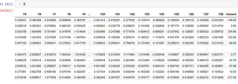

y.value_counts()

Class 0: 284315 Class 1: 492

# Standardize the features to have a mean of ~0 and a variance of 1
scaler = StandardScaler()
X_std = scaler.fit_transform(X)

To reduce the dimensionality of the data and visualize it better, PCA is applied to retain the two most important components. K-Means clustering is then performed on the PCA-transformed data. The number of clusters is set to two to calculate the distance of each data point to the cluster center as the anomaly score.

The number of clusters to choose from is rather arbitrary and most of the time it’s requires domain knowledge. There are methods to chose an optimal K which we won’t cover in this guide, but the reader can find them very easily.

In this case we choose K=2 and we will calculate distances from each data point to it’s corresponding centroid, we will assume that the farther the point from the centroid, the most likely it will be an anomaly.

# Apply PCA to reduce dimensions 
pca = PCA(n_components=2)
X_pca = pca.fit_transform(X_std)

import matplotlib.pyplot as plt

plt.figure(figsize=(10,7))
plt.scatter(X_pca[:,0], X_pca[:,1], c='blue', alpha=0.5)
plt.title('Scatter plot of the data before K-Means')
plt.xlabel('Principal Component 1')
plt.ylabel('Principal Component 2')
plt.show()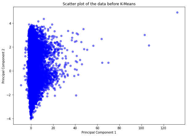

# Define the K-means model
kmeans = KMeans(n_clusters=2, random_state=42)

# Fit the model to the PCA-reduced data
kmeans.fit(X_pca)

# Predict the cluster labels: labels
labels = kmeans.predict(X_pca)

print(labels)

array([0, 0, 0, …, 1, 1, 1])

After fitting the K-Means model, the cluster labels for each data point are predicted and counted. A scatter plot can then be created to visualize the clusters along with the centroid.

plt.figure(figsize=(10,7))
plt.scatter(X_pca[:,0], X_pca[:,1], c=labels, cmap='viridis', alpha=0.5)
plt.scatter(kmeans.cluster_centers_[:,0], kmeans.cluster_centers_[:,1], s=300, c='red')
plt.title('Scatter plot of the data after K-Means')
plt.xlabel('Principal Component 1')
plt.ylabel('Principal Component 2')
plt.show()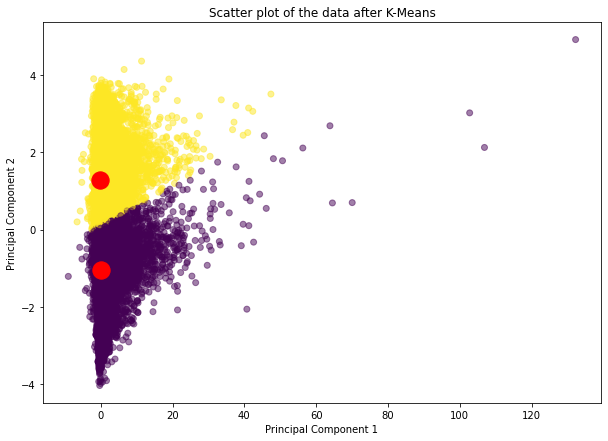

Next,

the code calculates the anomaly scores by computing the Euclidean distance from each point to its nearest cluster center.

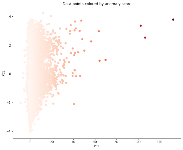
To create a more meaningful visualization, these scores are normalized and then mapped to colors on a red color scale. Darker shades of red indicate higher anomaly scores.

# Compute the distances to the cluster centers
distances = kmeans.transform(X_pca)

# Compute the anomaly score (distance to the closest centroid)
scores = distances.min(axis=1)

# Print the first 10 anomaly scores
print(scores[:10])

[1.52044216 1.12871036 2.34306172 0.76333104 0.47587477 1.10576802 0.65864807 0.19072126 0.09225452 0.89915189]

The final scatter plot shows the data points colored by their anomaly scores, providing an effective visualization of the potential anomalies in the dataset.

# Define the color map to convert scores to colors
import matplotlib.pyplot as plt
import matplotlib.cm as cm

# Create a color map that maps scores to colors
cmap = cm.get_cmap("Reds")

# Normalize the scores to the range [0, 1] for color mapping
normalized_scores = (scores - min(scores)) / (max(scores) - min(scores))

# Create a scatter plot of the PCA-transformed data with points colored by anomaly score
plt.figure(figsize=(10, 8))
plt.scatter(X_pca[:, 0], X_pca[:, 1], c=cmap(normalized_scores))
# plt.colorbar(label='Anomaly score')
plt.xlabel('PC1')
plt.ylabel('PC2')
plt.title('Data points colored by anomaly score')
plt.show()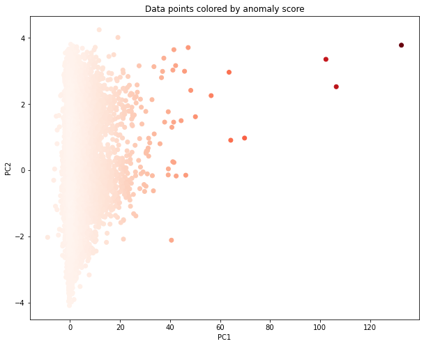

# Convert the normalized scores to a pandas series
normalized_scores_series = pd.Series(normalized_scores, name='Anomaly_Score')

# Concatenate the original DataFrame with the normalized scores
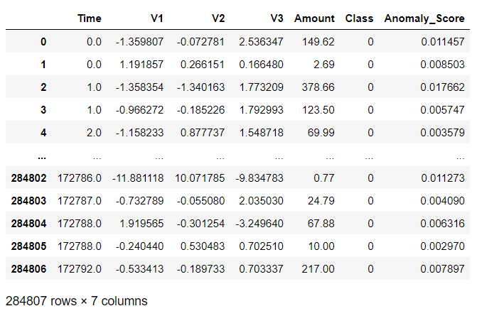
data_with_scores = pd.concat([data.reset_index(drop=True), normalized_scores_series], axis=1)data_with_scores[['Time','V1','V2','V3','Amount','Class', 'Anomaly_Score']]

Because we actually have the labels from the original dataset (which we haven’t used because this is unsupervised learning) we can use them to compare if the “Anomaly_Score” (distance from centroids) actually differ in Class 0 (normal transaction) vs Class 1 (fraudulent transactions). If we found the mean “Anomaly_Score” of Class 1 was statistically higher than the mean “Anomaly_Score” of Class 0, then our methodology could prove useful.

Here’s our dataset with the added Anomaly_Score column:

We can group by Class and calculate the mean Anomaly_Score:

grouped_data = data_with_scores.groupby('Class')['Anomaly_Score'].agg(['count', 'mean'])
print(grouped_data)

Class……..count …….mean 0 ………..284315 …..0.006233 1 …………….492 …..0.008536

The difference between the mean anomaly scores of the two classes is indeed noticeable, but in order to statistically test if this difference is significant, we can perform a two-sample t-test.

The two-sample t-test is used to determine if two population means are equal. The main assumptions of the test are that the two samples are independent, they are normally distributed, and they have the same variance.

Keep in mind that the t-test is sensitive to the normality assumption, and given that the scores are bounded in the interval [0, 1], they might not follow a normal distribution. You could use a non-parametric test, like Mann-Whitney U test, which does not require the assumption of normal distribution.

from scipy.stats import ttest_ind, mannwhitneyu

# Separating the scores for both classes
scores_class_0 = data_with_scores[data_with_scores['Class']==0]['Anomaly_Score']
scores_class_1 = data_with_scores[data_with_scores['Class']==1]['Anomaly_Score']

# Two-sample t-test
t_stat, p_val_t = ttest_ind(scores_class_0, scores_class_1)
print("t-test p-value: ", p_val_t)

# Mann-Whitney U test
u_stat, p_val_u = mannwhitneyu(scores_class_0, scores_class_1, alternative='two-sided')
print("Mann-Whitney U test p-value: ", p_val_u)

t-test p-value: 1.8125292456077149e-12 Mann-Whitney U test p-value: 1.7802027651503242e-24

A small p-value (typically ≤ 0.05) indicates strong evidence that the groups have different means, so you reject the null hypothesis that the means are the same.

Interpretation of Anomaly Scores by Class

By comparing the mean anomaly scores, we observe that the fraudulent transactions (Class ‘1’) have a higher mean anomaly score than non-fraudulent ones (Class ‘0’).

This is consistent with what we would expect: fraudulent transactions are, by nature, anomalous compared to regular transactions, and thus are more likely to be distant from the centroid of the clusters formed by K-Means.

Although the difference in mean scores between the two classes is not vast (0.008536 for fraudulent versus 0.006233 for non-fraudulent), it is statistically significant due to the large count of non-fraudulent transactions. This indicates that the K-Means clustering algorithm, as an unsupervised learning technique, provides a reasonable approach to distinguishing between regular and fraudulent transactions based on the anomaly scores.

However, it’s also important to remember that these anomaly scores are not binary classifications. They are better interpreted as a risk score that increases with the value of the score. Therefore, in a practical application, it would be useful to set an appropriate threshold for flagging transactions as potentially fraudulent.

Remember, K-Means is a simple and intuitive method for anomaly detection. For more complex datasets or higher performance needs, it might be necessary to use more advanced techniques. Nonetheless, K-Means provides a good starting point and a fundamental approach that is worthwhile to understand thoroughly.

See you in Chapter 6!

Chapter 6 code: https://github.com/gabrielpierobon/anomaly_detection/blob/main/Chapter%2005%20K-Means%20Clustering%20for%20anomaly%20detection.ipynb

Link to PDF Guide: https://drive.google.com/file/d/1g77lB2zeZGQUqIyPSb9Fr-uMyjmAG4j4/view?usp=drive_link