Statistical Techniques for Anomaly Detection (Part 1) Parametric and Non Parametric Tests

A carefully generated, thoroughly engineered resource for Data Scientists.

Part 1 of Chapter 02 from the Guide to Machine Learning for Anomaly Detection

Warning! Before you continue reading this article and all the articles that compose this guide, you must understand this was in part generated using OpenAI’s GPT 4 model. It started as a self learning project and I soon enough realized this could be really valuable to fellow data scientists. Because of this, I will release the entire guide for free alongside every chapter so you can directly go read the guide from the document so you don’t even need to give me reading time if you don’t want to.

Guide Index

In chapter 1, we immersed ourselves in understanding the fundamentals of anomaly detection, exploring what constitutes an anomaly, and the different types of anomalies:

point
contextual
collective

We realized that anomalies can indeed reveal crucial and insightful information in various fields, from finance to healthcare. Our journey now continues as we navigate the path of statistical techniques, which forms the bedrock of anomaly detection.

In this chapter, we will journey into the mathematical realm that underpins the world of anomaly detection. Given the dynamic nature of anomalies and the vast diversity of the datasets they can be found in, there exists a wide array of statistical techniques to discover them. In this chapter, we will demystify these techniques, beginning with an overview of parametric and non-parametric statistical tests. We will also explore the application of specific statistical tests, such as the Z-Score, Chi-Square Test, and Grubbs’ Test.

Each of these tests will be presented in a manner that elucidates their theoretical foundation and their applications in the real world. You will learn when and why each test is appropriate for certain kinds of datasets and anomalies. You will also see how these tests can help navigate the complex landscape of anomaly detection, enabling us to differentiate between a genuine anomaly and statistical noise.

Following this, we will move on to understanding univariate and multivariate anomalies.

Univariate anomalies pertain to datasets with only one variable, while
Multivariate anomalies are about datasets with multiple variables.

Here, the complexity expands as we start dealing with multiple dimensions. We will delve into the peculiarities of both types and learn about their distinct detection methods.

Through the course of this chapter, we aim to arm you with the statistical knowledge and practical skills required to master the art of anomaly detection. The goal is to empower you to not only understand the theoretical aspects of statistical anomaly detection but also to apply these learnings to real-world datasets with confidence.

As we embark on this mathematical adventure, remember that the value in anomaly detection lies not just in identifying the outliers, but also in interpreting these outliers.

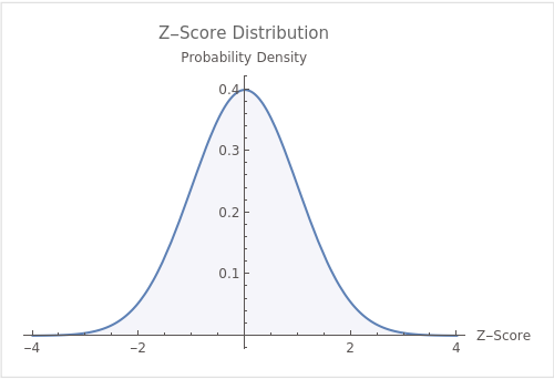
In the realm of statistics, tests are pivotal to decision-making and hypothesis testing. Statisticians and data scientists use these tests to discern significant patterns and relationships in the data, validate their assumptions, or debunk certain claims.

Broadly, these statistical tests can be classified into two categories:

parametric
non-parametric

Parametric tests

Parametric tests are grounded in certain assumptions about the characteristics of the data.

These tests assume that the data follows a specific distribution, typically a Gaussian or normal distribution. They also assume other conditions, such as homogeneity of variances and the independence of observations.

When these assumptions are met, parametric tests are powerful tools for hypothesis testing and are relatively sensitive to the nuances of the data.

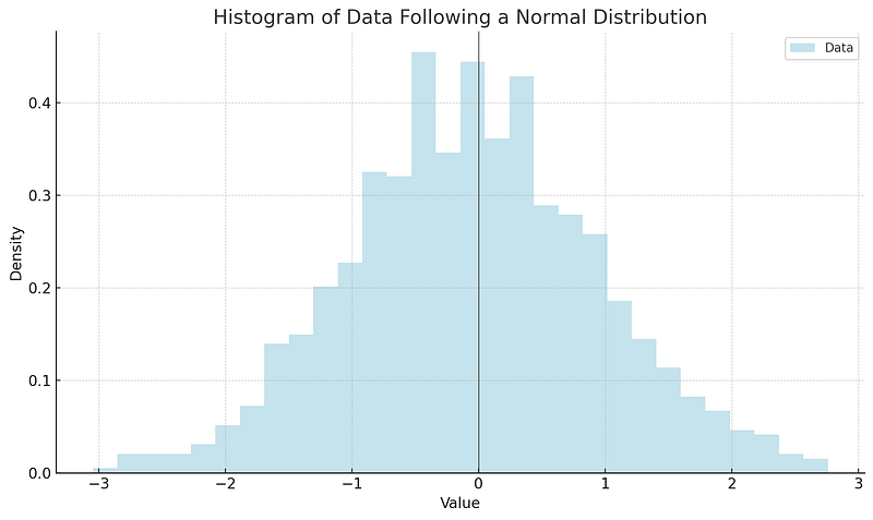
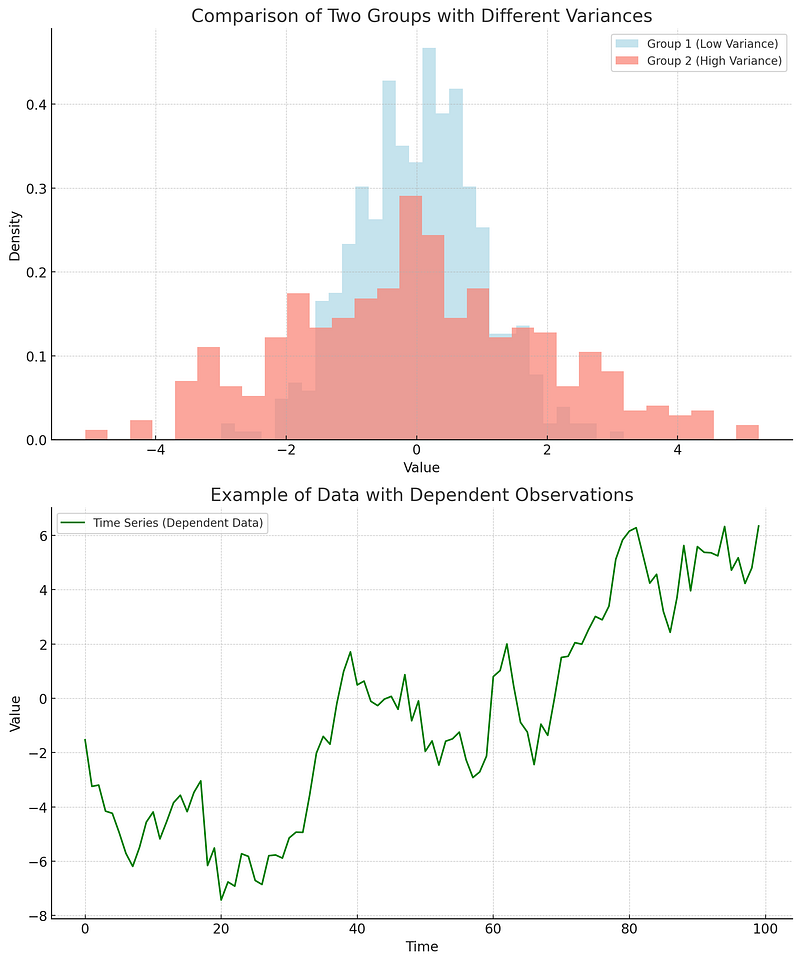
The histogram above shows the synthetic data we generated, which follows a normal (or Gaussian) distribution. As you can see, the data is bell-shaped, which is characteristic of a normal distribution.

The visualizations provided highlight the two assumptions:

Homogeneity of Variances: The top plot compares two groups with different variances. Ideally, when conducting statistical tests that assume homogeneity, the variances of the groups should be similar. Here, “Group 1” has a lower variance (it’s more narrowly distributed), while “Group 2” has a higher variance (it’s more spread out).
Independence of Observations: The bottom plot showcases a time series, which is an example of dependent data. Each data point (after the first) is dependent on the previous data points. In tests that assume independent observations, such data would not be appropriate.

For anomaly detection,

parametric methods come in handy in situations where the data adheres to a known distribution.

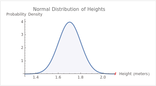
For instance, a dataset of human heights in a certain population might be expected to follow a normal distribution. If we then come across an unusually low or high value (say, a height of 2.5 meters), we can leverage parametric tests to quantify how anomalous this data point is relative to the rest of the dataset.

Common parametric tests include the Z-Test, T-Test, Analysis of Variance (ANOVA), and Linear Regression.

Each of these tests caters to different scenarios and data setups. For instance, the Z-Test and T-Test are used to compare the means of one or two groups, respectively, while ANOVA is used to compare the means of three or more groups. Linear Regression, on the other hand, is a predictive modeling technique that assumes a linear relationship between the independent and dependent variables.

Coding Time: Implementing and Interpreting Parametric Tests in Python

We can use Python to perform these parametric tests. Here are some examples using the scipy and statsmodels libraries:

Z-Test

The Z-Test is used when the data is normally distributed and the population variance is known. However, in practice, it’s often used when the sample size is large, regardless of the distribution.

'''
In this example, we first generate two groups of random data from a 
normal distribution. The np.random.normal function generates random 
numbers from a normal distribution with a specified mean and standard 
deviation. We then perform a Z-Test using the stats.ttest_ind function 
from the scipy library. This function returns two values: the Z-Score 
and the P-Value. The Z-Score is a measure of how many standard deviations 
an element is from the mean. The P-Value is used in hypothesis testing 
to help you support or reject the null hypothesis. It represents the 
probability that the results of your test occurred at random. If p-value 
is less than 0.05, we reject the null hypothesis.
'''

from scipy import stats
import numpy as np

# Generate random data
np.random.seed(0)
group1 = np.random.normal(0.1, 1.0, 1000)
group2 = np.random.normal(0.2, 1.0, 1000)

# Perform Z-Test
z_score, p_value = stats.ttest_ind(group1, group2)
print(f"Z-Score: {z_score}, P-Value: {p_value}")

Z-Score: -3.631948749571147 P-Value: 0.00028837831940553923

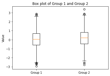
The Z-Score of -3.63 indicates that the mean of `group1` is lower than that of `group2`. The very low P-Value of approximately 0.00029 suggests that this difference is not due to random chance. Since this P-Value is much less than the common threshold of 0.05, we conclude that there’s a statistically significant difference between the two groups’ means.

T-Test

The T-Test is used when the data is normally distributed but the population variance is unknown. It’s typically used for smaller sample sizes.

'''
This example is very similar to the Z-Test example. The difference is that 
we are using smaller sample sizes (30 instead of 1000). The T-Test is more 
appropriate than the Z-Test when the sample size is small. The interpretation 
of the T-Score and P-Value is the same as for the Z-Test.
'''

# Generate random data
np.random.seed(0)
group1 = np.random.normal(0.1, 1.0, 30)
group2 = np.random.normal(0.2, 1.0, 30)

# Perform T-Test
t_score, p_value = stats.ttest_ind(group1, group2)
print(f"T-Score: {t_score}, P-Value: {p_value}")

T-Score: 2.421173504228532 P-Value: 0.018620022435273602

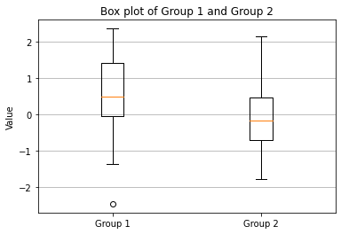
The T-Test was conducted to determine if there was a statistically significant difference between the means of group1 and group2. The resulting T-Score of 2.421 suggests a difference between the two groups, and the P-Value of 0.0186 (which is less than the common alpha level of 0.05) indicates that this difference is statistically significant. Therefore, we can conclude that the means of the two groups are likely not the same.

ANOVA (Analysis of Variance)

ANOVA is used to compare the means of three or more groups.

'''
In this example, we generate three groups of random data and perform an 
ANOVA test using the stats.f_oneway function. The F-Score is a measure of 
how much the means of each group differ from the mean of the overall data 
set. The P-Value is the same as in the previous examples. If the P-Value 
is less than 0.05, we can reject the null hypothesis that the means of 
all groups are equal.
'''

# Generate random data
np.random.seed(0)
group1 = np.random.normal(0.1, 1.0, 30)
group2 = np.random.normal(0.2, 1.0, 30)
group3 = np.random.normal(0.3, 1.0, 30)

# Perform ANOVA
f_score, p_value = stats.f_oneway(group1, group2, group3)
print(f"F-Score: {f_score}, P-Value: {p_value}")

F-Score: 3.0583006692442627 P-Value: 0.052048465538565784

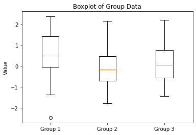
The ANOVA test was conducted to determine if there are any statistically significant differences between the means of the three groups. With an F-Score of 3.0583 and a P-Value of 0.052, the results are just above the commonly used significance threshold of 0.05. This means that while there are some differences between the group means, they aren’t statistically significant at the 0.05 level. Hence, we cannot confidently reject the null hypothesis that the means of all three groups are equal.

Linear Regression

Linear Regression is a predictive modeling technique that assumes a linear relationship between the independent and dependent variables.

import statsmodels.api as sm

# Generate random data
np.random.seed(0)
X = np.random.normal(0, 1.0, 100)
Y = 2*X + np.random.normal(0, 0.1, 100)

# Add constant to input variables
X = sm.add_constant(X)

# Perform Linear Regression
model = sm.OLS(Y, X)
results = model.fit()
print(results.summary())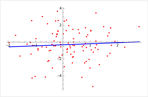

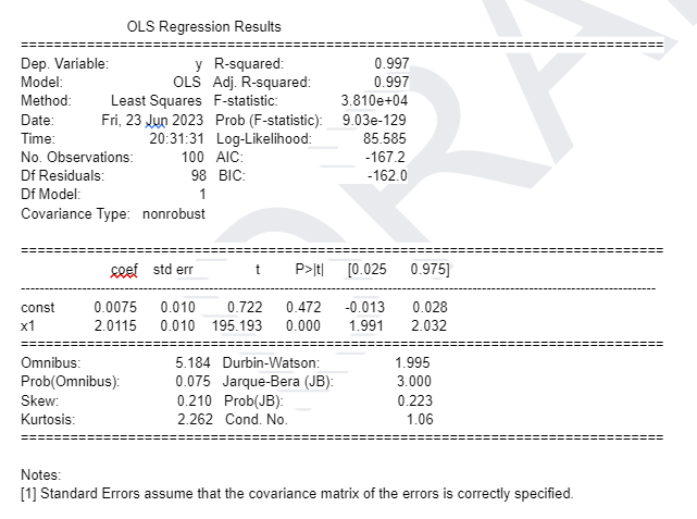
In this example, we first generate random data for our independent variable X and dependent variable Y. The relationship between X and Y is linear, with Y being twice X plus some normally distributed noise.

We then add a constant to our independent variables. This is necessary because the statsmodels’ OLS function doesn’t add an intercept to our model by default.

We then create a model using the sm.OLS function and fit the model to our data using the fit method.

Finally, we print a summary of our model. This summary includes a lot of information, but some key values to look at are:

coef: This is the estimated coefficient for the corresponding variable. In our case, we should see a value close to 2 for X1 (our X variable) and a value close to 0 for the constant (since we didn’t add a constant to Y when generating the data).
std err: This is the standard error of the estimate of the coefficient. Smaller values are better.
P>|t|: This is the p-value for the hypothesis test that the coefficient is zero, given the data. If this value is less than 0.05, we can reject the null hypothesis and conclude that the variable does have an effect on the dependent variable.
R-squared: This is the coefficient of determination, a statistical measure that shows the proportion of the variance for a dependent variable that’s explained by an independent variable or variables in a regression model. If it’s 1, it means the variables are perfectly correlated, i.e., with no variance at all. A low value, on the other hand, shows poor correlation.

Please note that these are basic examples and real-world scenarios would require additional steps such as data cleaning, checking assumptions, and interpreting results.

Non-parametric tests

Non-parametric tests, in contrast, do not assume a specific distribution for the data. These tests are distribution-free and are thus less powerful but more flexible than their parametric counterparts.

They can be applied to a wide variety of data types, including ordinal and nominal data, and are robust to outliers and non-normality.

In the context of anomaly detection,

non-parametric methods are beneficial when the data does not conform to a known or well-defined distribution, or when the nature of the distribution is not known.

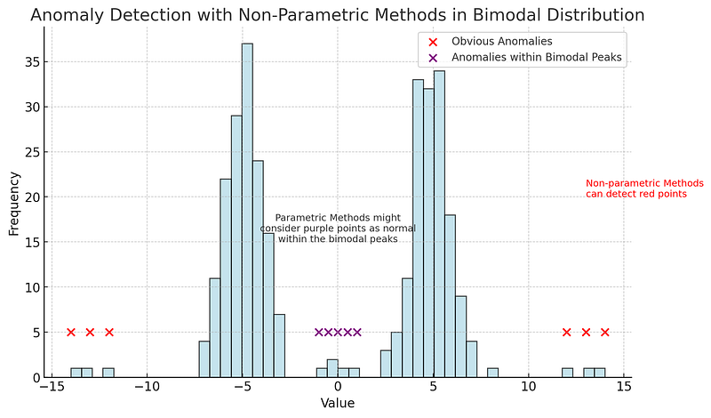
These methods rely on techniques such as ranking or bootstrapping and are generally more robust against anomalies.

Popular non-parametric tests include the Chi-Square Test, Mann-Whitney U Test, Kruskal-Wallis Test, and Spearman’s Rank Correlation. These tests, like their parametric counterparts, serve different purposes and apply to different types of data and research questions. For instance, the Chi-Square Test is often used to test for associations between categorical variables, while Spearman’s Rank Correlation measures the strength and direction of association between two ranked variables.

Coding Time: Hands-On with Non-Parametric Tests Using Python

Chi-Square Test

The Chi-Square Test is often used to test for associations between categorical variables. Here is an example of how to use it in Python using scipy.stats.chi2_contingency.

'''
In this case, the p-value will give us the probability that we would see 
these results given the null hypothesis of no association between the 
categorical variables. If this p-value is below a certain significance 
level (often 0.05), we reject the null hypothesis and conclude that there 
is a statistically significant association between the variables.
'''

import numpy as np
from scipy.stats import chi2_contingency

# Define a 2-D contingency table
table = np.array([[10, 20, 30],
                  [20, 40, 60]])

chi2, p, dof, ex = chi2_contingency(table)

print(f"Chi-Square statistic: {chi2}")
print(f"P-value: {p}")
print(f"Degrees of freedom: {dof}")
print(f"Expected table: \n{ex}")

Chi-Square statistic: 0.0 P-value: 1.0 Degrees of freedom: 2 Expected table: [[10. 20. 30.] [20. 40. 60.]]

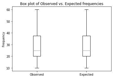
The Chi-Square test results show that there is no significant association between the rows and columns of the provided contingency table. The Chi-Square statistic is 0.0, indicating a perfect fit between the observed and expected frequencies. This is further confirmed by the p-value of 1.0, which suggests that the observed and expected frequencies are identical. Thus, the data does not provide evidence to reject the null hypothesis of independence between the variables.

We can check what happens if we change our values like this:

import numpy as np
from scipy.stats import chi2_contingency

# Define a 2-D contingency table
table = np.array([[10, 20, 30],
                  [999, 1, 100]])

chi2, p, dof, ex = chi2_contingency(table)

print(f"Chi-Square statistic: {chi2}")
print(f"P-value: {p}")
print(f"Degrees of freedom: {dof}")
print(f"Expected table: \n{ex}")

Chi-Square statistic: 468.2352766713519 P-value: 2.108635697963909e-102 Degrees of freedom: 2 Expected table: [[ 52.18965517 1.0862069 6.72413793] [956.81034483 19.9137931 123.27586207]]

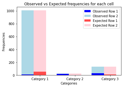
The Chi-Square test indicates a significant association between the rows and columns of the table, with a Chi-Square statistic of 468.24 and an extremely low p-value (2.11e-102), far below any conventional significance level (e.g., 0.05). This means that the observed frequencies in the table differ significantly from what would be expected under the assumption of independence between the two classifications.

Mann-Whitney U Test

The Mann-Whitney U Test is used to compare the distributions of two independent groups. Here’s how you can use it with the scipy.stats.mannwhitneyu function:

'''
In this example, a low p-value suggests that the distributions of the two 
groups are significantly different.
'''

from scipy.stats import mannwhitneyu

# Two groups of data
group1 = [1, 2, 3, 4, 5]
group2 = [6, 7, 8, 9, 10]

# Perform the Mann-Whitney U Test
u, p = mannwhitneyu(group1, group2)

print(f"U statistic: {u}")
print(f"P-value: {p}")

U statistic: 0.0 P-value: 0.006092890177672406

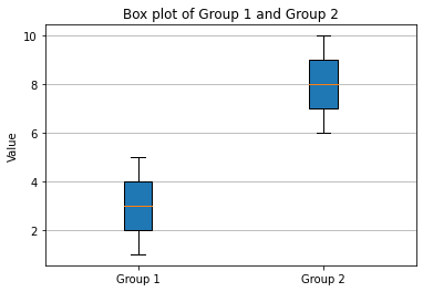
The Mann-Whitney U test indicates a significant difference between the two groups, with a U statistic of 0.0 and a p-value of 0.0061. Given that the p-value is less than the common significance threshold (0.05), we can reject the null hypothesis and infer that the distributions of the two groups are not the same, with group1 having typically lower values than group2.

Again, if we make some changes:

# Two groups of data
group1 = [1, 2, 3, 4, 5]
group2 = [2, 1, 4, 3, 5]

# Perform the Mann-Whitney U Test
u, p = mannwhitneyu(group1, group2)

print(f"U statistic: {u}")
print(f"P-value: {p}")

U statistic: 12.5 P-value: 0.45776498668838594

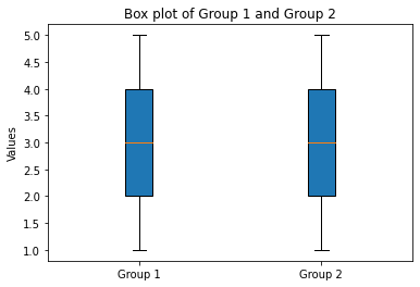
The Mann-Whitney U Test was performed to compare the distributions of two independent groups, `group1` and `group2`. The resulting U statistic is 12.5, and the associated p-value is approximately 0.458. This p-value suggests that there’s no statistically significant difference between the distributions of the two groups at a conventional significance level (e.g., 0.05). In other words, we do not have sufficient evidence to say that one group tends to have larger or smaller values than the other.

Kruskal-Wallis Test

The Kruskal-Wallis Test is a non-parametric version of ANOVA, used to compare the distributions of three or more independent groups. It’s implemented as scipy.stats.kruskal.

'''
Like the previous tests, a low p-value suggests that at least one of the 
distributions is different from the others.
'''

from scipy.stats import kruskal

# Three groups of data
group1 = [1, 2, 3, 4, 5]
group2 = [1, 2, 3, 1, 2]
group3 = [5, 6, 7, 8, 9]

# Perform the Kruskal-Wallis Test
h, p = kruskal(group1, group2, group3)

print(f"H statistic: {h}")
print(f"P-value: {p}")

H statistic: 9.962909090909088 P-value: 0.006864071189260182

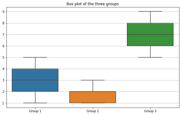
The Kruskal-Wallis test evaluates whether there’s a statistically significant difference between the medians of three or more independent groups. In this case, the H statistic is 9.96 and the p-value is approximately 0.0069. Since the p-value is below the common alpha level of 0.05, it suggests that there’s a statistically significant difference in the median values of at least one of the groups when compared to the others. Thus, we have evidence to reject the null hypothesis that all groups have the same median.

Spearman’s Rank Correlation

Spearman’s Rank Correlation is used to measure the strength and direction of the association between two ranked variables. It’s implemented as scipy.stats.spearmanr.

'''
In this example, the correlation coefficient tells us how strongly the 
two variables are associated. A p-value below a certain significance 
level suggests that the correlation is statistically significant.
'''

from scipy.stats import spearmanr

# Two sets of data
data1 = [1, 2, 3, 4, 5]
data2 = [5, 6, 7, 8, 7]

# Perform Spearman's Rank Correlation
corr, p = spearmanr(data1, data2)

print(f"Spearman's correlation: {corr}")
print(f"P-value: {p}")

Spearman’s correlation: 0.8207826816681233 P-value: 0.08858700531354381

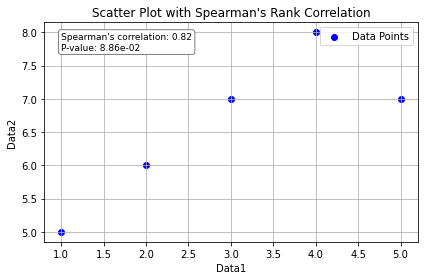
The Spearman’s correlation coefficient of 0.82 suggests a strong positive association between the two data sets. However, with a p-value of 0.089, this correlation is not statistically significant at the conventional 0.05 level, indicating that we cannot confidently assert that the observed relationship is not due to random chance.

It’s important to understand that parametric and non-parametric tests are not inherently superior to each other but rather serve different purposes.

The choice between the two depends on the nature of your data, the research question at hand, and the assumptions you are willing and able to make about your data. Furthermore, the boundary between parametric and non-parametric can sometimes be blurred. For instance, some techniques such as Kernel Density Estimation or K-Nearest Neighbors can be tweaked to behave either like parametric or non-parametric methods, depending on the chosen parameters.

In the upcoming sections, we will delve into some of these tests in detail. We will cover the underlying theory, the assumptions and conditions they require, how they can be used for anomaly detection, and how to implement them using Python. By understanding these tests and learning how to apply them, you will be well-equipped to handle a variety of anomaly detection scenarios, whether your data follows a known distribution or not.

Chapter 2 continues in the next article!

Link to Chapter 2 code : https://github.com/gabrielpierobon/anomaly_detection/blob/main/Chapter%2002%20Statistical%20Techniques%20for%20Anomaly%20Detection.ipynb

Link to PDF Guide: https://drive.google.com/file/d/1g77lB2zeZGQUqIyPSb9Fr-uMyjmAG4j4/view?usp=drive_link