Introduction to Machine Learning for Anomaly Detection (Part 2)

A carefully generated, thoroughly engineered resource for Data Scientists.

Part 2 of Chapter 03 from the Guide to Machine Learning for Anomaly Detection

Warning! Before you continue reading this article and all the articles that compose this guide, you must understand this was in part generated using OpenAI’s GPT 4 model. It started as a self learning project and I soon enough realized this could be really valuable to fellow data scientists. Because of this, I will release the entire guide for free alongside every chapter so you can directly go read the guide from the document so you don’t even need to give me reading time if you don’t want to.

Guide Index

We continue were we left off in Part 1…

Coding Time: Supervised Learning with Random Forest Classifier

In this section, we will use a Supervised Learning method, specifically Random Forest Classifier, for anomaly detection. This technique will be employed on a synthetically generated dataset, which will contain two classes — ‘Normal’ and ‘Anomaly’. By performing Random Forest Classification, we will attempt to classify whether a datapoint is normal or an anomaly.

The Random Forest algorithm is a type of ensemble learning method that operates by constructing multiple decision trees at training time and outputting the class that is the mode of the classes (classification) or mean prediction (regression) of the individual trees.

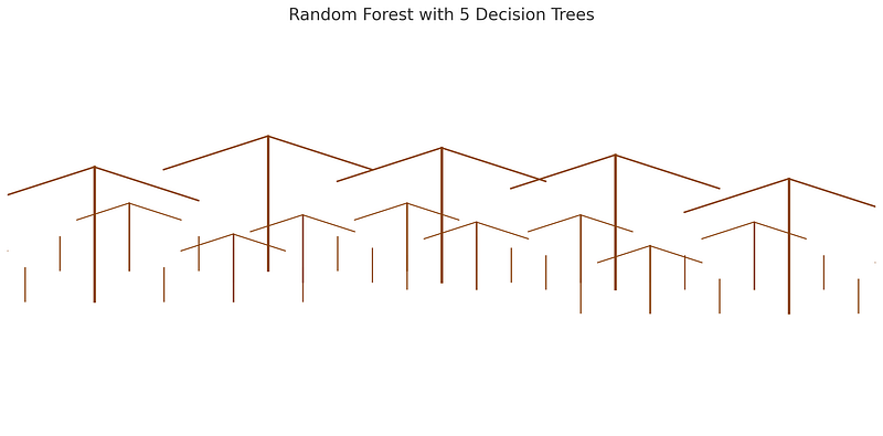
I don’t know why I liked this representation so much! LOL ;)

Here’s a step-by-step breakdown of how the Random Forest algorithm works:

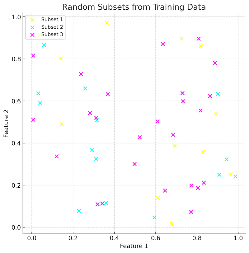
Random Subsets: The algorithm starts by selecting random subsets of the data from the training set. Each subset is used to train a decision tree. This randomness ensures that each decision tree is trained on different data and helps avoid overfitting to the training data.

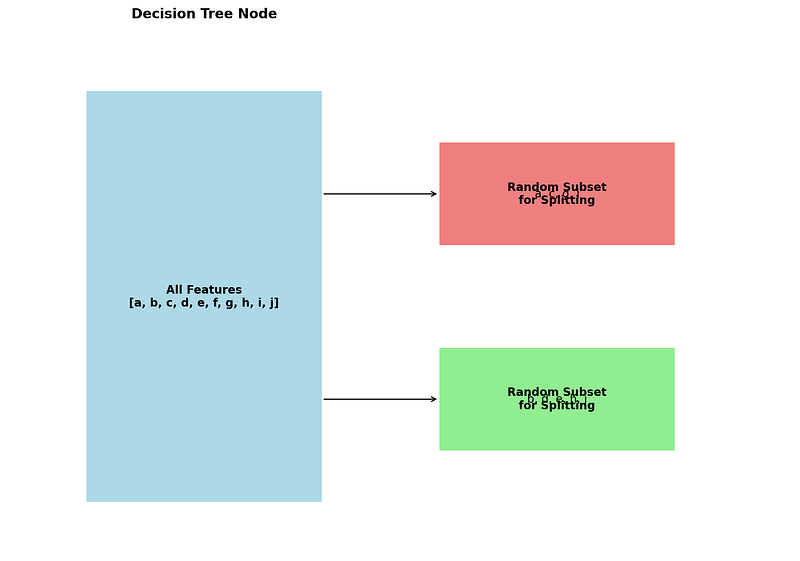
2. Splitting Nodes: For each decision tree, a subset of features is selected at each node to determine the best split. Instead of looking at all features to find the best split (as in a regular decision tree), it looks at a random subset of them. This is the ‘random’ aspect of a ‘Random Forest’ and injects more randomness into the model.

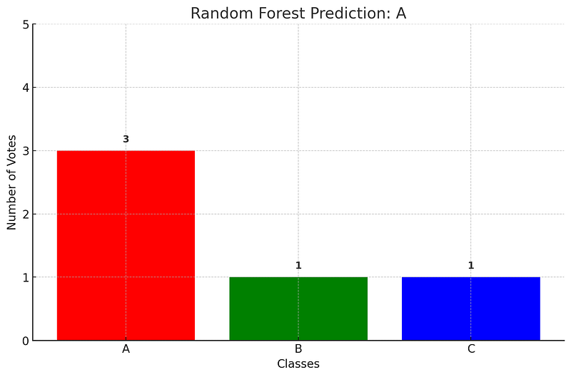
3. Prediction: After a large number of trees are generated, each tree “votes” or “predicts” for a class, and the class receiving the most votes over all trees in the forest is predicted by the random forest.

4. Aggregation: For regression problems, the average prediction of all the trees is considered as the final result. For classification, the majority voting system is used, i.e., the prediction that has the most votes from all the decision trees is considered the final prediction.

This algorithm is popular because it’s a powerful tool with a few great features:

The algorithm can be used for both regression and classification tasks.
It reduces overfitting by averaging the result from many decision trees.
It handles a large proportion of missing values and maintains accuracy for missing data.
It can estimate which of your variables are important in the classification, offering a feature importance estimate.

The synthetic dataset we will utilize here is generated using the make_classification function from Scikit-learn, which creates a binary classification problem. Class ‘0’ represents normal data points, and class ‘1’ represents anomalies. We are creating an imbalanced dataset where anomalies constitute the minority class (only about 1% of the data points), simulating real-world anomaly detection scenarios.

We will then split the dataset into a training set and a test set, train a Random Forest Classifier model using the training data, and evaluate it on the test data. Evaluation will be carried out using various performance metrics such as the confusion matrix, precision, recall, F1-score, and ROC AUC score.

import numpy as np
import pandas as pd
from sklearn.datasets import make_classification
from sklearn.ensemble import RandomForestClassifier
from sklearn.model_selection import train_test_split
from sklearn.metrics import classification_report, roc_auc_score
from sklearn.metrics import plot_confusion_matrix
import matplotlib.pyplot as plt

# Generate a random n-class classification problem
X, y = make_classification(n_samples=10000, n_features=20, n_informative=2, n_redundant=10,
                           n_clusters_per_class=1, weights=[0.99], flip_y=0, random_state=4)

# Split the dataset into training and test datasets
X_train, X_test, y_train, y_test = train_test_split(X, y, test_size=0.2, random_state=42)

# Create and fit the model
model = RandomForestClassifier(n_estimators=100)
model.fit(X_train, y_train)

# Predict the test set results
y_pred = model.predict(X_test)

# Evaluate the model
print("Classification Report: \n", classification_report(y_test, y_pred))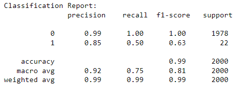

Here’s a brief summary of the performance metrics and what they mean in this context:

Class 0 (Normal transactions)

Precision: The model is 99% precise when it predicts a transaction is normal, meaning that 99% of the transactions it identified as normal are indeed normal.
Recall: The model has a recall of 100% for normal transactions, which means it correctly identified all of the normal transactions in the dataset.
F1-Score: The F1-score is the harmonic mean of precision and recall. An F1-score reaches its best value at 1 (perfect precision and recall) and worst at 0. For normal transactions, the F1-score is 1, suggesting excellent model performance for normal transactions.

Class 1 (Anomalous transactions)

Precision: The model is 85% precise when it predicts a transaction is anomalous. This means that 85% of the transactions it flagged as anomalies were indeed anomalies.
Recall: However, the model only identified 50% of the actual anomalies in the dataset, resulting in a recall of 0.50. This means it failed to identify half of the anomalies, which is a significant limitation.
F1-Score: The F1-score for anomalous transactions is 0.63, which is lower than the F1-score for normal transactions. This is because of the lower recall for anomalies, which pulls down the F1-score.

Overall Accuracy

The overall accuracy of the model is 99%, indicating that it made correct predictions for 99% of the instances in the dataset. However, given the imbalanced nature of this dataset (where anomalies are rare), accuracy can be a misleading metric.

The lower recall for anomalies (class 1) suggests that the model is less capable of identifying anomalous transactions compared to normal ones. This could be due to the significant imbalance in the dataset, where anomalous transactions are much rarer than normal ones. The model might have overfitted to the normal transactions, which are abundant in the data, at the expense of correctly identifying the anomalies.

In practical terms, depending on the specific costs associated with false positives (flagging a normal transaction as an anomaly) and false negatives (missing an anomaly), you might want to adjust your model, perhaps by resampling the dataset to have more equal class distribution, or by adjusting the decision threshold of the classifier.

# Plot the confusion matrix
plot_confusion_matrix(model, X_test, y_test)
plt.show()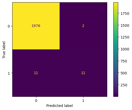

Area Under the Curve and Receiver Operating Characteristic (ROC) Curve

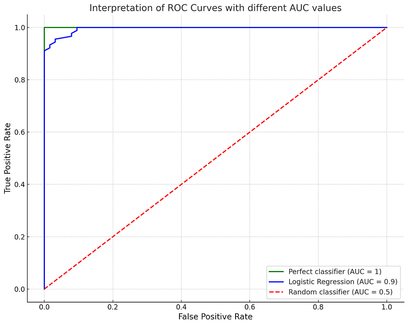
This ROC Curve is an illustration, does not belong to this specific example.

The AUC, or Area Under the Curve, is a performance measurement for classification problems that tells us how much a model is capable of distinguishing between classes.

It is used in conjunction with the

Receiver Operating Characteristic (ROC) curve, which plots the true positive rate (sensitivity) against the false positive rate (1 — specificity) at various threshold settings.

The AUC value lies between 0 and 1. A model whose predictions are 100% wrong has an AUC of 0, while a model whose predictions are 100% correct has an AUC of 1. Therefore, the closer the AUC to 1, the better.

Here’s a more detailed interpretation:

AUC = 1, the classifier is able to perfectly distinguish between all the Positive and the Negative class points correctly. If the AUC had been 0, then the classifier would be predicting all Negatives as Positives, and all Positives as Negatives.
0.5 < AUC < 1, there is a high chance that the classifier will be able to distinguish the positive class values from the negative class values. This is so because the classifier is able to detect more numbers of True positives and True negatives than False negatives and False positives.
AUC = 0.5, then the classifier is not able to distinguish between Positive and Negative class points. Meaning it is predicting random outputs (either positive or negative) and, as a result, we will get equal numbers of false positives and true positives, which makes the AUC 0.5.

In summary, the higher the AUC value, the better the model is at predicting 0s as 0s and 1s as 1s.

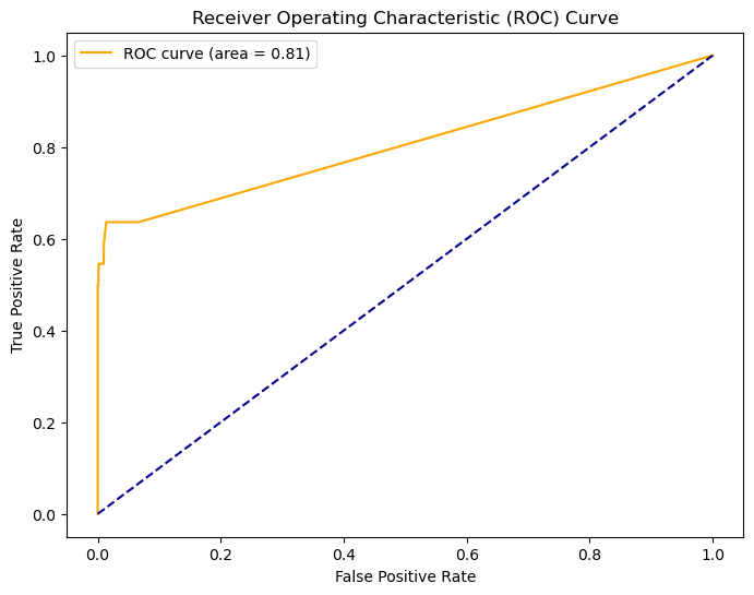
Here’s how you can plot the Receiver Operating Characteristic (ROC) curve and calculate the Area Under the Curve (AUC) score for the Random Forest classifier in our anomaly detection scenario:

You will need to use the roc_curve and roc_auc_score functions from sklearn.metrics, as well as matplotlib for plotting.

from sklearn.metrics import roc_curve, roc_auc_score
import matplotlib.pyplot as plt

# Predict probabilities for the test data.
y_probs = model.predict_proba(X_test)

# Keep only the positive class
y_probs = y_probs[:, 1]

# Compute the ROC curve
fpr, tpr, thresholds = roc_curve(y_test, y_probs)

# Compute the AUC score
auc_score = roc_auc_score(y_test, y_probs)
print(f"AUC Score: {auc_score}")

# Create a plot
plt.figure(figsize=(8,6))
plt.plot(fpr, tpr, color='orange', label='ROC curve (area = %0.2f)' % auc_score)
plt.plot([0, 1], [0, 1], color='darkblue', linestyle='--')
plt.xlabel('False Positive Rate')
plt.ylabel('True Positive Rate')
plt.title('Receiver Operating Characteristic (ROC) Curve')
plt.legend()
plt.show()

AUC Score: 0.8050027576063976

Feature Importance

Feature importance refers to techniques that assign a score to input features based on how useful they are at predicting a target variable.

In a random forest, every tree will give an importance score to each feature. We can calculate the average score across all trees to obtain the overall importance of each feature.

Here’s how you can print the feature importances:

# Since our example uses a numpy array instead of a features dataset, let's name our features with a number
feature_names = []
for feature_nbr in range(1, X.shape[1]+1):
    feature_names.append(f"feature_{feature_nbr}")

# Extract feature importances
importances = model.feature_importances_
importance_series = pd.Series(importances, index=feature_names)
importance_series.sort_values(ascending=False, inplace=True)

print(importance_series)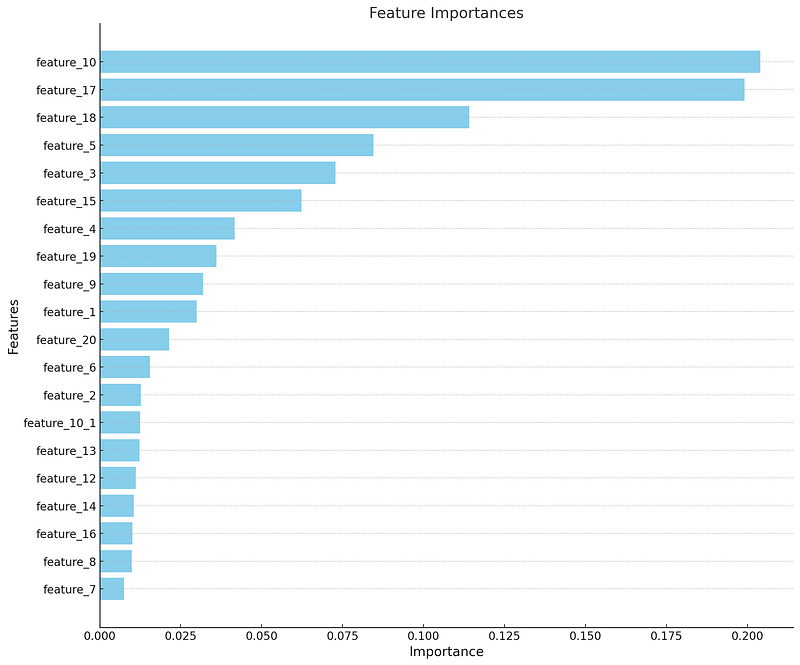

The feature importances output provided by a Random Forest Classifier gives you an idea about which features are most influential when it comes to making decisions about the target class.

Looking at the list of feature importances, we can see that `feature_10` and `feature_17` are the two most important features for the random forest model, with importances of approximately 0.204 and 0.199 respectively. This means that these two features contribute the most to the decisions of the random forest model when distinguishing between normal and anomalous transactions.

Following `feature_10` and `feature_17`, the next most important feature is `feature_18` with an importance of around 0.114. It’s quite a bit lower than the first two, but it still carries a significant weight.

The remaining features exhibit a steady decrease in importance, with each having a decreasing influence on the model’s decision process. Some of the features, such as `feature_7` and `feature_8` have very low importance scores, suggesting they may not contribute significantly to the model’s predictions.

It’s important to note that these importances do not indicate whether the features have a positive or negative impact on the predicted class — only the magnitude of their impact.

Also, they are specific to the trained model and the dataset it was trained on. Changing the model configuration or the data could lead to different feature importances.

In practical terms, you might use this information to gain insights into the underlying data and the model’s behavior, or to simplify your model by eliminating features that don’t contribute significantly to the prediction. However, do keep in mind that even features with lower importance can still play a critical role in prediction when interacting with other features.

Coding Time: Supervised Learning with Support Vector Classifier

Support Vector Machines (SVMs) are a set of supervised learning methods used for classification, regression, and outliers detection. For classification tasks, which is what we’re interested in here,

SVMs use a technique called the “kernel trick” to transform data and then based on these transformations, it finds an optimal boundary between the possible outputs.

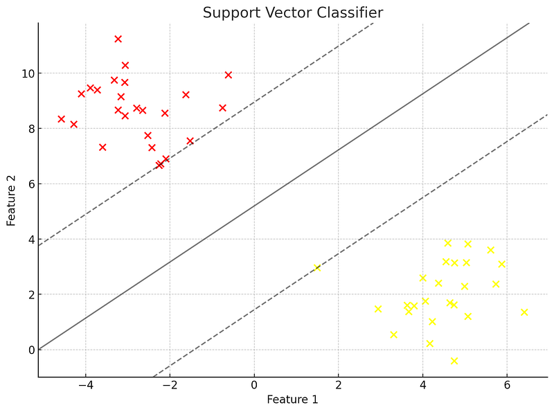
Essentially, the model creates a line or a hyperplane which separates the data into classes. The best line or hyperplane is the one that has the largest distance to the nearest training data points of any class (so-called functional margin). Hence, in a two-dimensional space, SVMs would divide the plots into two separated areas divided by a straight line.

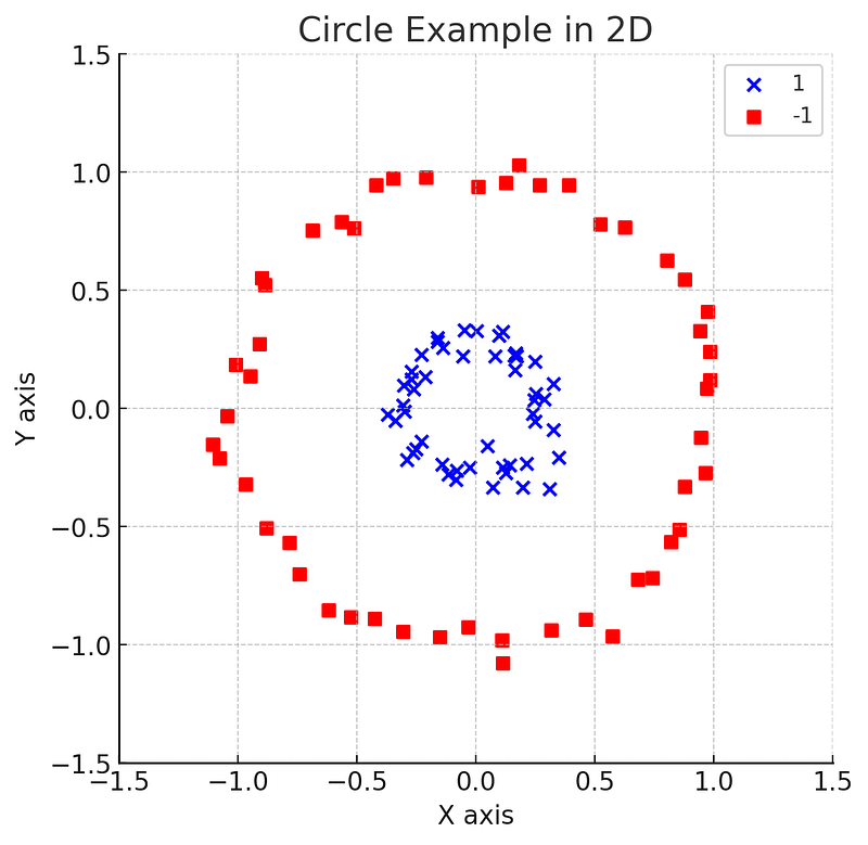
The Circle Example: Demonstrating the SVM Kernel Trick

In this example, we have a set of data points that are distributed in two regions: - Inside a circle (represented by blue x’s) - Outside the circle (represented by red squares)

In the 2D representation, it’s evident that there is no straight line (linear decision boundary) that can separate these two classes of data points. This is a classic instance of a non-linear classification problem.

Support Vector Machines (SVM) provide a powerful technique called the “kernel trick” to handle such non-linear data. Instead of trying to fit a non-linear decision boundary in the original space,

the kernel trick implicitly maps the data to a higher-dimensional space where it might be linearly separable.

For our Circle Example, we used the Radial Basis Function (RBF) kernel, a popular choice for SVM. This kernel effectively transformed our 2D data into a 3D space.

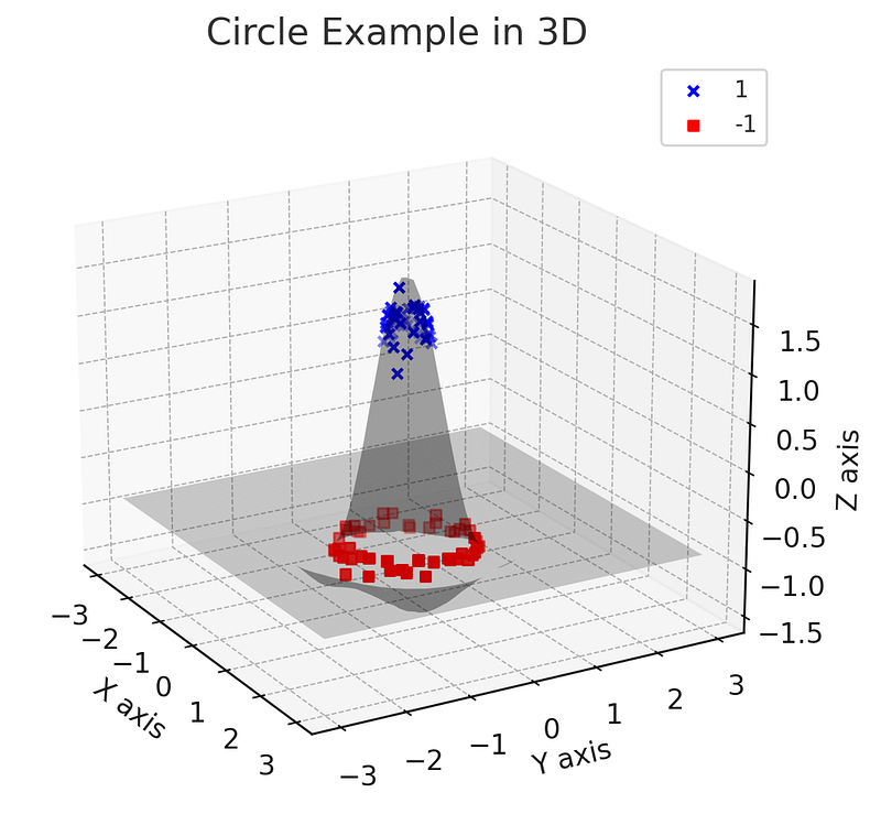
In the transformed 3D space, our once non-linearly separable data now appeared in such a manner that a flat plane (a linear decision boundary in 3D) could easily separate the two classes. The data points that were once inside the circle in the 2D space were now “above” this plane in the 3D space, and those outside the circle were “below” the plane.

This transformation didn’t change the inherent relationships between data points but provided a new perspective (or dimension) to view the data, allowing for linear separation.

Let’s revisit our previous example using a Support Vector Classifier (SVC). We’re still trying to identify anomalies in our data, but this time, we’re going to use an SVC instead of a Random Forest.

import numpy as np
import pandas as pd
from sklearn.datasets import make_classification
from sklearn.ensemble import RandomForestClassifier
from sklearn.model_selection import train_test_split
from sklearn.metrics import classification_report, roc_auc_score
from sklearn.metrics import plot_confusion_matrix
import matplotlib.pyplot as plt

# Generate a random n-class classification problem
X, y = make_classification(n_samples=10000, n_features=20, n_informative=2, n_redundant=10,
                           n_clusters_per_class=1, weights=[0.99], flip_y=0, random_state=4)

# Split the dataset into training and test datasets
X_train, X_test, y_train, y_test = train_test_split(X, y, test_size=0.2, random_state=42)

from sklearn.svm import SVC
from sklearn.metrics import classification_report, confusion_matrix, roc_auc_score, roc_curve

# create a SVC model
model_svc = SVC(kernel='linear', probability=True, random_state=42)

# train the model
model_svc.fit(X_train, y_train)


# make predictions
y_pred_svc = model_svc.predict(X_test)
y_probs_svc = model_svc.predict_proba(X_test)[:, 1]  # keep probabilities for the positive outcome only

print("Classification Report: ")
print(classification_report(y_test, y_pred_svc))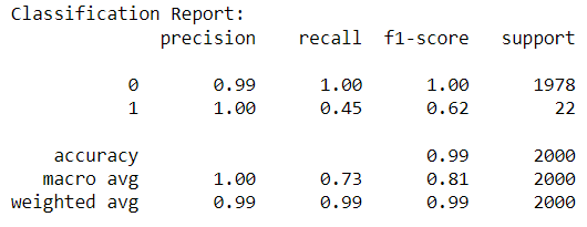

# Plot the confusion matrix
plot_confusion_matrix(model_svc, X_test, y_test)
plt.show()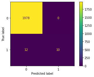

The classification report provides a breakdown of each class by precision, recall, f1-score and support showing excellent results.

Precision is the ability of a classifier not to label an instance positive that is actually negative. For each class, it is defined as the ratio of true positives to the sum of true and false positives. In this case, for class 0, precision is 0.99, meaning that 99% of the instances that the model labeled as class 0 were actually class 0. For class 1, the precision is perfect 1.00, so every instance that the model predicted as class 1 was indeed class 1.
Recall is the ability of a classifier to find all positive instances. For each class it is defined as the ratio of true positives to the sum of true positives and false negatives. The recall for class 0 is 1.00, indicating that the model identified all instances of class 0 correctly. The recall for class 1 is 0.45, indicating that the model was only able to correctly identify 45% of the class 1 instances.
F1-score: The F1 score is a weighted harmonic mean of precision and recall such that the best score is 1.0 and the worst is 0.0. F1 scores are lower than accuracy measures as they embed precision and recall into their computation. For class 0, the F1-score is 1.00, indicating excellent precision and recall. For class 1, the F1-score is 0.62, which is a relatively good score, considering the imbalanced nature of the dataset, and the difficulties inherent in correctly identifying class 1 instances.
Support: Support is the number of actual occurrences of the class in the specified dataset. For class 0, support is 1978, and for class 1, support is 22. Imbalanced support in the training data may indicate structural weaknesses in the reported scores of the classifier and could indicate the need for stratified sampling or rebalancing.

In the context of our anomaly detection task, this model is showing great precision, but it is not as good in terms of recall for the anomalous class (class 1).

This means that while the model is very accurate when it does detect an anomaly, it only catches 45% of the anomalies. This result might be acceptable in some contexts where false positives are a significant concern, but it could be a problem if it is essential to detect as many anomalies as possible.

It is also worth comparing these results to those obtained with the Random Forest model. The Random Forest model had a recall of 0.50 for class 1, slightly higher than the SVC’s recall of 0.45. However, the SVC model had perfect precision for class 1, while the Random Forest model’s precision for class 1 was 0.85.

This suggests that the SVC may be more precise but slightly less sensitive than the Random Forest model. The choice between these models would depend on whether precision or recall is more important for your specific application.

from sklearn.metrics import roc_curve, roc_auc_score
import matplotlib.pyplot as plt

# Predict probabilities for the test data.
y_probs = model_svc.predict_proba(X_test)

# Keep only the positive class
y_probs = y_probs[:, 1]

# Compute the ROC curve
fpr, tpr, thresholds = roc_curve(y_test, y_probs)

# Compute the AUC score
auc_score = roc_auc_score(y_test, y_probs)
print(f"AUC Score: {auc_score}")

# Create a plot
plt.figure(figsize=(8,6))
plt.plot(fpr, tpr, color='orange', label='ROC curve (area = %0.2f)' % auc_score)
plt.plot([0, 1], [0, 1], color='darkblue', linestyle='--')
plt.xlabel('False Positive Rate')
plt.ylabel('True Positive Rate')
plt.title('Receiver Operating Characteristic (ROC) Curve')
plt.legend()
plt.show()

AUC Score: 0.9055290008272819

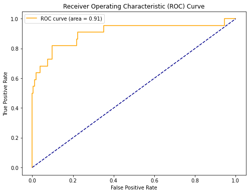
The AUC score for the Support Vector Classifier (SVC) model is approximately 0.91. This means that there is a 91% chance that the model will be able to distinguish between a positive class and a negative class. This result is pretty good.

See you in chapter 4!

Link to Chapter 3 code: https://github.com/gabrielpierobon/anomaly_detection/blob/main/Chapter%2003%20Introduction%20to%20Machine%20Learning%20for%20Anomaly%20Detection.ipynb

Link to PDF Guide: https://drive.google.com/file/d/1g77lB2zeZGQUqIyPSb9Fr-uMyjmAG4j4/view?usp=drive_link