Isolation Forest for Anomaly Detection

A carefully generated, thoroughly engineered resource for Data Scientists.

Chapter 07 from the Guide to Machine Learning for Anomaly Detection

Warning! Before you continue reading this article and all the articles that compose this guide, you must understand this was in part generated using OpenAI’s GPT 4 model. It started as a self learning project and I soon enough realized this could be really valuable to fellow data scientists. Because of this, I will release the entire guide for free alongside every chapter so you can directly go read the guide from the document so you don’t even need to give me reading time if you don’t want to.

Guide Index

In this chapter, we delve into an exciting approach for anomaly detection — the Isolation Forest method. This method is unique and diverges significantly from the traditional clustering or distance-based techniques that we have explored so far.

The main idea of Isolation Forest revolves around the concept of ‘isolating’ anomalies instead of profiling normal data points.

Anomalies are data points that are few and different, which should make them easier to ‘isolate’ compared to normal instances. Isolation Forest leverages this principle to detect anomalies in a remarkably efficient and effective manner.

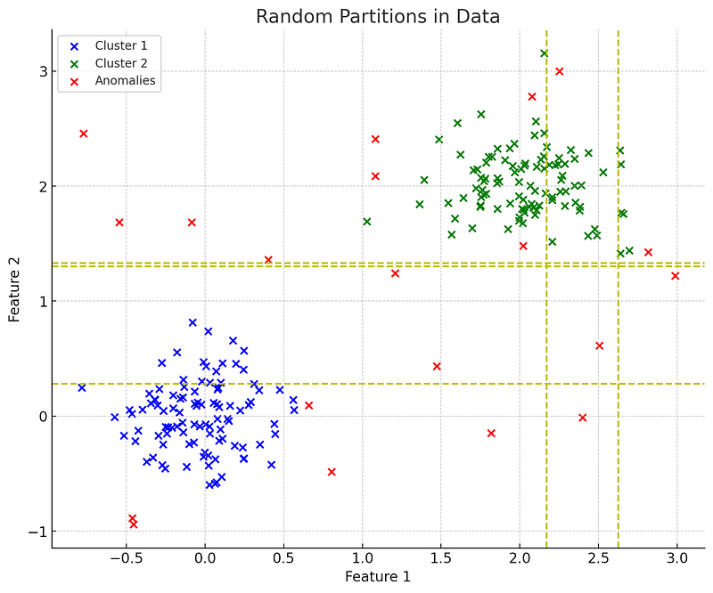
This approach isolates anomalies by randomly selecting a feature and then randomly selecting a split value between the maximum and minimum values of the selected feature. The logic here is that anomalous data points require fewer random partitions to be isolated compared to normal points, as they are fewer in number and different from the rest.

One of the key benefits of Isolation Forest is its efficiency.

The number of partitions required is a measure of the anomaly score, and this can be calculated with a low computational cost.

It is also indifferent to the underlying distribution of the data,

making it a versatile tool for anomaly detection tasks in various domains.

Isolation Forest has been used effectively in a number of areas such as fraud detection, intrusion detection in networks, and medical anomaly detection. In this chapter, we will explore how to implement and apply Isolation Forest for anomaly detection. We will discuss the intuition behind it, its implementation, and we will demonstrate its usage through practical examples.

Intuition Behind the Isolation Forest Algorithm

The name “Isolation Forest” might already give you a clue about how the algorithm operates. In essence, it’s all about isolating observations, and as the name suggests, it does so by using a forest of trees. Let’s unravel this.

Just as humans are adept at identifying objects that deviate from the norm visually, Isolation Forest identifies anomalies based on the principle that anomalies are data points that are few and different.

This means anomalies are ‘isolatable’ in fewer steps compared to normal points.

For example, imagine you’re playing the game “Guess Who?” with a group of characters. If there’s a character that is distinctly different from the others (say, the only one wearing glasses), you’ll be able to isolate this character in fewer questions.

This principle extends to the Isolation Forest algorithm.

The algorithm builds an ensemble of ‘Isolation Trees’ for the data set and splits subsets randomly by selecting a random feature and a random split value.

Since anomalous data points are less frequent, they tend to appear in smaller, isolated branches on the isolation trees.

In contrast, normal instances of the dataset will often share branches that are both longer and deeper within the tree.

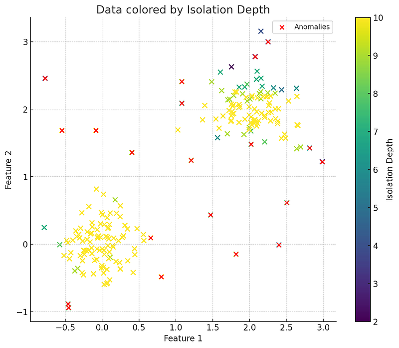
The number of splits required to isolate a sample is equivalent to the path length from the root node to the terminating node. This path length, averaged over a forest of such random trees, is a measure of normality and our decision function.

Shorter path lengths indicate that the instance is likely to be an anomaly.

Theory of Isolation Forest

Now that we understand the intuition behind the Isolation Forest algorithm, let’s delve a bit deeper into its theoretical background.

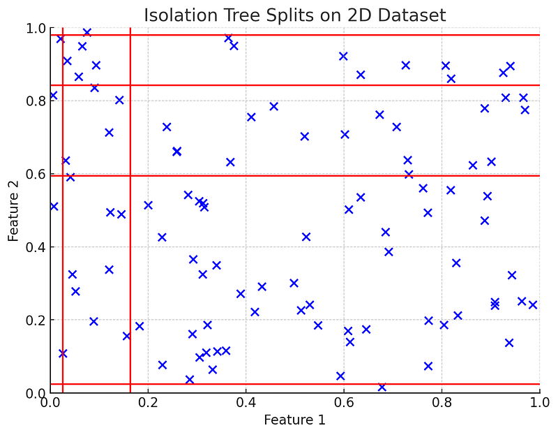
An iTree is similar to a decision tree, but with the primary goal of isolating every data point. Instead of splitting nodes to maximize or minimize some criterion, the iTree splits nodes randomly.

Construction

For a given data point: 1. Randomly select a feature f from the dataset. 2. Randomly select a split value v between the minimum and maximum values of feature f. 3. Split the dataset into two subsets:

S1: Points with f less than v
S2: Points with f greater than or equal to v

Repeat this process recursively for each subset.

Termination

The recursive process terminates when:

The tree reaches a maximum height, defined as ⌈log2(n)⌉ where n is the number of instances.
All instances at the node are isolated.

Path Length, ℎ(x)

The path length is the number of edges from the root node to the terminating node for a particular instance. For an anomaly, this path is expected to be short because it’s more easily isolated.

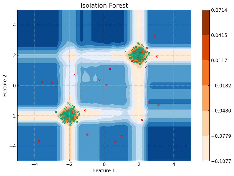
Blue points represent the data points. Red lines depict the decision boundaries introduced by the Isolation Tree.

Anomaly Score

An anomaly score s(x) is defined as:

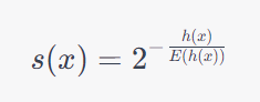
Where: - h(x) is the path length of instance x in the iTree. - E(h(x)) is the average path length in the tree.

Instances with scores closer to 1 are more likely to be anomalies.

Anomalies will typically have shorter path lengths in the iTree due to their inherent isolatability.

This score is calculated for each tree in the forest, and an average anomaly score is assigned to each instance.

If all instances are isolated before reaching the height limit, the tree is considered balanced. However, if a majority of instances are isolated at smaller heights, the tree is considered unbalanced, indicating the presence of anomalies.

It is important to note that Isolation Forest works well in high-dimensional datasets and doesn’t require a normality assumption in the data, making it a versatile and robust anomaly detection technique.

The plot shows the decision boundary of the Isolation Forest (light blue for inliers and dark blue for outliers) and the data points. The white points are the training observations, the green points are new regular observations, and the red points are new abnormal observations. As you can see, the Isolation Forest does a good job of distinguishing between normal and abnormal observations. The abnormal observations generally have a higher anomaly score (shown by the darker blue region) compared to the normal observations.

Coding Time — Detecting Credit Card Fraud with Isolation Forest

In this section, we’ll be implementing the Isolation Forest algorithm to detect anomalies in our credit card transaction dataset. Specifically, we’re going to build an Isolation Forest model and use it to predict which transactions are anomalous — these could potentially be fraudulent transactions.

# Import necessary libraries
import pandas as pd
from sklearn.ensemble import IsolationForest
from sklearn.preprocessing import StandardScaler

# Load the dataset
data = pd.read_csv('creditcard.csv')

# Separate out the features and labels
X = data.drop('Class', axis=1)
y = data['Class']

# Standardize the features to have a mean of ~0 and a variance of 1
scaler = StandardScaler()
X_std = scaler.fit_transform(X)

# Define the model
model = IsolationForest(contamination=0.0017)

# Fit the model to the data
model.fit(X_std)

# Use the model to predict anomalies in the data
y_pred = model.predict(X_std)

# Map the predicted values from {-1,1} to {0,1}
y_pred = [1 if x == -1 else 0 for x in y_pred]

# Add the predictions to the original dataframe
data['Isolation Forest Anomaly Prediction'] = y_pred

# Create a crosstab to view the predicted and actual class distributions
pd.crosstab(data['Class'], data['Isolation Forest Anomaly Prediction'])

The Isolation Forest model returns a prediction of -1 for anomalies and 1 for normal data points. Therefore, we map these back to 0 and 1 to match the original class labels.

After fitting the model and making predictions, we add these predictions back into the original dataframe. This allows us to directly compare our model’s anomaly predictions to the actual class labels.

Finally, we create a cross-tabulation, or contingency table, to view the distribution of predicted and actual classes. This helps us understand how well our model has performed in detecting anomalous, potentially fraudulent transactions.

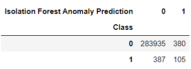
The cross-tabulation of the Isolation Forest predictions against the actual class labels provides us a simple way to evaluate the model’s performance.

Results

The number 283,935 in the intersection of `Class 0` (normal transactions) and `Isolation Forest Anomaly Prediction 0` shows that the model correctly identified 283,935 normal transactions.
The number 105 in the intersection of `Class 1` (fraudulent transactions) and `Isolation Forest Anomaly Prediction 1` shows that the model correctly identified 105 fraudulent transactions as anomalies.
The number 380 in the intersection of `Class 0` (normal transactions) and `Isolation Forest Anomaly Prediction 1` shows that the model incorrectly identified 380 normal transactions as anomalies. These are false positives.
The number 387 in the intersection of `Class 1` (fraudulent transactions) and `Isolation Forest Anomaly Prediction 0` shows that the model failed to identify 387 fraudulent transactions and classified them as normal. These are false negatives.

It seems that the model is doing a good job in correctly identifying normal transactions (with very few false positives), but it is missing a number of fraudulent transactions (high false negatives). In a fraud detection scenario, it’s typically more acceptable to have false positives (flagging normal transactions as potentially fraudulent) rather than false negatives (missing fraudulent transactions), as the latter would mean fraudulent activity goes unnoticed.

These findings suggest that while our Isolation Forest model is somewhat effective in identifying anomalies in this dataset, there’s room for improvement, especially in its ability to catch more fraudulent cases. This could potentially be achieved through fine-tuning the model parameters or employing additional feature engineering techniques.

We’re not interested here in boosting its performance, we’ll leave it up to you!

See you in Chapter 8!

Code for Chapter 7: https://github.com/gabrielpierobon/anomaly_detection/blob/main/Chapter%2007%20Isolation%20Forest%20for%20Anomaly%20Detection.ipynb

Link to PDF Guide: https://drive.google.com/file/d/1g77lB2zeZGQUqIyPSb9Fr-uMyjmAG4j4/view?usp=drive_link