
How to Swing Algo-Trade Tech Stocks using the Qullamaggie's Breakouts — 1. NVIDIA

- The objective of this post is to resolve a risk-return trade-off of a swing algo-trading strategy in Python that aims at capturing short or medium gains in a growth tech stock such as NVIDIA (NDAQ: NVDA).
- Following the Qullamaggie’s breakout strategy, we take on board a simple yet effective scanner in Python that algorithmically scans for high-growth, and sideways price actions.
- Let’s embark on the journey!
- Setting the working directory PATH, the stock ticker and importing basic libraries
import os
os.chdir('PATH')    # Set working directory
os. getcwd()
import numpy as np
import pandas as pd
import yfinance as yf
import seaborn as sns
import matplotlib.pyplot as plt

ticker='NVDA'def trend_filter(prices: pd.core.series.Series,
growth_4_min: float = 25.,
growth_12_min: float = 50.,
growth_24_min: float = 80.) -> np.array:
growth_func = lambda x: 100*(x.values[-1]/x.min() - 1)
growth_4 = df['Close'].rolling(20).apply(growth_func) > growth_4_min
growth_12 = df['Close'].rolling(60).apply(growth_func) > growth_12_min
growth_24 = df['Close'].rolling(120).apply(growth_func) > growth_24_min
return np.where(
growth_4 | growth_12 | growth_24,
1,
0,
)
if __name__ == '__main__':
df = yf.download(ticker)
df.loc[:, 'trend_filter'] = trend_filter(df['Close'])
df.dropna()
df_trending = df[df['trend_filter'] == 1] - Time series smoothing using an explicit FD method and checking for consolidation
def explicit_heat_smooth(prices: np.array,
                         t_end: float = 5.0) -> np.array:

    k = 0.1 # Time spacing, must be < 1 for numerical stability

    P = prices

    t = 0
    while t < t_end:
        P = k*(P[2:] + P[:-2]) + P[1:-1]*(1-2*k)


        P = np.hstack((
            np.array([prices[0]]),
            P,
            np.array([prices[-1]]),
        ))
        t += k

    return P


def check_consolidation(prices: np.array,
                        perc_change_days: int,
                        perc_change_thresh: float,
                        check_days: int) -> int:


    prices = explicit_heat_smooth(prices)


    perc_change = prices[perc_change_days:]/prices[:-perc_change_days] - 1

    consolidating = np.where(np.abs(perc_change) < perc_change_thresh, 1, 0)


    if np.sum(consolidating[-check_days:]) > 0:
        return 1
    else:
        return 0


def find_consolidation(prices: np.array,
                       days_to_smooth: int = 50,
                       perc_change_days: int = 5,
                       perc_change_thresh: float = 0.015,
                       check_days: int = 5) -> np.array:

    res = np.full(prices.shape, np.nan)

    for idx in range(days_to_smooth, prices.shape[0]):
        res[idx] = check_consolidation(
            prices = prices[idx-days_to_smooth:idx],
            perc_change_days = perc_change_days,
            perc_change_thresh = perc_change_thresh,
            check_days = check_days,
        )

    return res

if __name__ == '__main__':

    df = yf.download(ticker)
    df.loc[:, 'consolidating'] = find_consolidation(df['Close'].values)
df.dropna()- Plotting the binary ‘consolidating’ if df[‘Close’] > 600 USD
dff=df[df['Close'] > 600]
fig = plt.figure(figsize=(15, 7))
scal=5e4
plt.scatter(dff.index,dff['consolidating'],s=dff["Volume"]/scal,c=dff["Close"],cmap='viridis')
plt.colorbar()
plt.xlabel('Date')
plt.grid()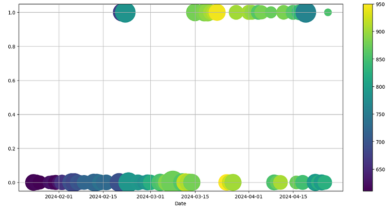
- Creating and plotting the ‘filtered’ binary column
df = yf.download('NVDA')
df.loc[:, 'consolidating'] = find_consolidation(df['Close'].values)
df.loc[:, 'trend_filter'] = trend_filter(df['Close'])
df.loc[:, 'filtered'] = np.where(
    df['consolidating'] + df['trend_filter'] == 2,
    True,
    False,
)
dff1=df[df['Close'] > 600]
ig = plt.figure(figsize=(15, 7))
scal=5e4
plt.scatter(dff1.index,dff1['trend_filter'],s=dff["Volume"]/scal,c=dff["Close"],cmap='viridis')
plt.colorbar()
plt.xlabel('Date')
plt.grid()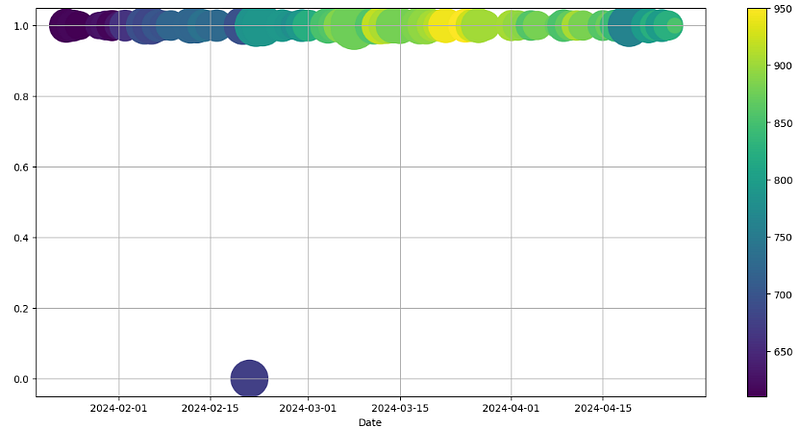
- Final visualization of the ‘filtered’ column based on the binary value — close price before/after filtering
df.index = pd.DatetimeIndex(data=df.index, tz='US/Eastern')
dft = pd.DataFrame({'DateTime': df.index})
# selecting rows based on condition
df1 = df[df['filtered'] > 0]
df0 = df[df['filtered'] < 1]
dft1 = pd.DataFrame({'DateTime': df1.index})
dft0 = pd.DataFrame({'DateTime': df0.index})
plt.figure(figsize=(12,10))
scal=5e5
plt.scatter(df0.index, df0["Close"],color='red',s=df0["Volume"]/scal,alpha=0.4)
plt.scatter(df1.index, df1["Close"],color='green',s=df1["Volume"]/scal,alpha=0.4)
plt.xlabel("Date")
plt.ylabel("Price $")

plt.legend(["Close" , "Filtered"], facecolor='bisque',
           loc='upper center', bbox_to_anchor=(0.5, -0.08),
           ncol=2)
plt.grid()
plt.show()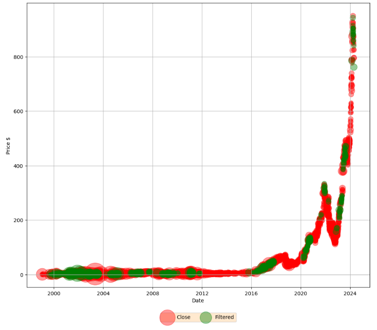
- Optionally checking DateTime Index and shape of our data
print(df0.index)
DatetimeIndex(['1999-01-22 00:00:00-05:00', '1999-01-25 00:00:00-05:00',
               '1999-01-26 00:00:00-05:00', '1999-01-27 00:00:00-05:00',
               '1999-01-28 00:00:00-05:00', '1999-01-29 00:00:00-05:00',
               '1999-02-01 00:00:00-05:00', '1999-02-02 00:00:00-05:00',
               '1999-02-03 00:00:00-05:00', '1999-02-04 00:00:00-05:00',
               ...
               '2024-03-27 00:00:00-04:00', '2024-04-09 00:00:00-04:00',
               '2024-04-10 00:00:00-04:00', '2024-04-11 00:00:00-04:00',
               '2024-04-16 00:00:00-04:00', '2024-04-18 00:00:00-04:00',
               '2024-04-22 00:00:00-04:00', '2024-04-23 00:00:00-04:00',
               '2024-04-24 00:00:00-04:00', '2024-04-25 00:00:00-04:00'],
              dtype='datetime64[ns, US/Eastern]', name='Date', length=5643, freq=None)

df0.shape
(5643, 9)

print(df1.index)
DatetimeIndex(['1999-09-09 00:00:00-04:00', '1999-09-10 00:00:00-04:00',
               '1999-09-13 00:00:00-04:00', '1999-10-06 00:00:00-04:00',
               '1999-10-08 00:00:00-04:00', '1999-12-01 00:00:00-05:00',
               '1999-12-02 00:00:00-05:00', '1999-12-03 00:00:00-05:00',
               '1999-12-06 00:00:00-05:00', '1999-12-07 00:00:00-05:00',
               ...
               '2024-04-02 00:00:00-04:00', '2024-04-03 00:00:00-04:00',
               '2024-04-04 00:00:00-04:00', '2024-04-05 00:00:00-04:00',
               '2024-04-08 00:00:00-04:00', '2024-04-12 00:00:00-04:00',
               '2024-04-15 00:00:00-04:00', '2024-04-17 00:00:00-04:00',
               '2024-04-19 00:00:00-04:00', '2024-04-26 00:00:00-04:00'],
              dtype='datetime64[ns, US/Eastern]', name='Date', length=714, freq=None

df1.shape
(714, 9)- Examining the zoomed version of the above plot if df[‘Close’] > 600 USD
rslt_df0 = df0.loc[df0['Close'] > 600]
rslt_df1 = df1.loc[df1['Close'] > 600]
plt.figure(figsize=(10,6))
scal=5e5
plt.scatter(rslt_df0.index, rslt_df0["Close"],color='red',s=rslt_df0["Volume"]/scal,alpha=0.4)
plt.scatter(rslt_df1.index, rslt_df1["Close"],color='green',s=rslt_df1["Volume"]/scal,alpha=0.4)
plt.xlabel("Date")
plt.ylabel("Price $")

plt.legend(["Close" , "Filtered"], facecolor='bisque',
           loc='upper center', bbox_to_anchor=(0.5, -0.08),
           ncol=2)
plt.grid()
plt.show()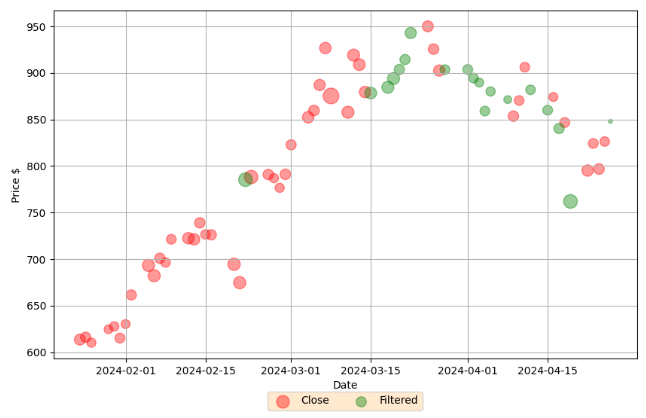
- Breakouts are certainly key indicators of trend shifts, providing traders with chances for financial gain.
- It is therefore useful to compare these indicators to NVDA candlesticks with other trading indicators.
Conclusions
- Today we have talked about the swing breakout algo-trading algorithm in Python.
- To be a successful swing trader, we must minimize losses and maximize profits by holding a position either long or short for more than one trading session, but usually not longer than several weeks or a couple of months.
- Our current swing algo-trading strategy is based on the Qullamaggie methodology that combines technical analysis market indicators and risk management strategies.
- We have shown how to profit from short-term price movements in the NVDA price swings using this methodology.
Explore More
- Backtesting Algo-Trading Strategies, FinTech Analysis & Portfolio Optimization: NVDA, AMD, INTC, MSI vs S&P 500 Benchmark
- Backtesting the NVIDIA Scalping Strategy with SPY Benchmark & VaR Simulations
- Backtesting Hybrid CI & MACD Trading Strategies for NVIDIA
- NVIDIA Algo-Trading: VaR, Q-Q Plots & Stochastic Simulations
- A Deeper Look at NVIDIA KST Algo-Trading Signals & Backtesting
- NVIDIA 14–20 RSI-BB Algo-Trading
- Portfolio Optimization of 4 Major Techs: Markowitz, Sharpe, VaR & CAPM
- Algo-Trading NVIDIA with Donchian Channels
- Algo-Trading NVIDIA with ADX & RSI Indicators
- Deploying Streamlit Stock Fundamental Analysis App — NVIDIA Example
- An Algo-Trading Sneak Peek at Top AI-Powered Growth Stocks — 1. NVIDIA
- A Market-Neutral Strategy
- NVIDIA Returns-Drawdowns MVA & RNN Mean Reversal Trading
- IQR-Based Log Price Volatility Ranking of Top 19 Blue Chips
- Returns-Volatility Domain K-Means Clustering and LSTM Anomaly Detection of S&P 500 Stocks
- NVIDIA Rolling Volatility: GARCH & XGBoost
- The Qullamaggie’s TSLA Breakouts for Swing Traders
- The Qullamaggie’s OXY Swing Breakouts
References
- A Simple Way to Scan for Breakout Candidates Using Python
- Scripting the Swing: To filter stocks based on setup
- Trading Breakout Strategies — the Dos and Don’ts
- Breakout Trading Strategy Used by Professional Traders
- What is Swing Trading?
- Swing Trading
- How to Swing Trade Tech Stocks (by Scott Redler / @RedDogT3)


