
Backtesting Algo-Trading Strategies, FinTech Analysis & Portfolio Optimization: NVDA, AMD, INTC, MSI vs S&P 500 Benchmark

Image template by @ondostudios via Canva.
- The objective of this project is to perform robust backtesting and portfolio optimization of 4 tech game-changers (NVDA, AMD, INTC & MSI) vs the S&P 500 benchmark.
- Backtesting is a risk-free validation of (algo-)trading strategies, ensuring they are adaptable to various market conditions. The process of backtesting involves selecting relevant historical data, applying the technical analysis strategy, and then analyzing its potential profitability.
- Portfolio Optimization (PO) aims at resolving the risk-return trade-off by maximizing the return for every additional unit of risk taken in the portfolio. PO utilizes advanced financial models to generate optimal investment portfolios balancing desired returns with acceptable risk levels. PO takes into account a variety of factors: market trends, asset correlations, technical indicators, etc.
- What about the 4 top-rated tech stocks to be discussed in the sequel?
- Chip companies have been in focus this year due to the massive opportunity created by the generative artificial intelligence ambitions of tech giants following the success of OpenAI’s ChatGPT.
- Advanced Micro Devices (NASDAQ:AMD), Nvidia (NASDAQ:NVDA), and Intel (NASDAQ:INTC) are known to be the best chip stocks as per Wall Street experts.
- Motorola Solutions, Inc. (NYSE: MSI) is the leading global provider of mission critical communication services. MSI serves more than 100,000 public safety and commercial customers across more than 100 countries. MSI recently announced the launch of cutting-edge solutions with advanced capabilities.
- The present study entails a comprehensive fintech analysis of these 4 celebrated stocks in terms of their business performance and overall financial health over recent years.
- Using the proposed set of Python open-source tools and techniques to analyze historical stock data and financial statements can help investors make more informed business decisions to predict and improve ROI.
- Let’s get to the heart of the matter!
Basic Installations & Imports
- Set up a Lean, Robust Data Science Environment with Miniconda and Conda-Forge. You can find the latest version of Miniconda here.
- Go to C:\Users\miniconda3\condabin (in cmd)
- Use the
conda info --envscommand to access a list of all available conda environments for your user profile. - Use the following command to create a new conda environment
- conda create — name
python==X.X.X - Use the activate command
conda activate <env_name>- Use the
conda install -c conda-forge jupyterinstall the jupyter package. - Run
jupyter notebook - Use deactivate command upon exiting
conda deactivate- Within the Jupyter Notebook IDE:
- Setting up the working directory YOURPATH
import os
os.chdir('YOURPATH')    # Set working directory
os. getcwd() - Installing and importing Python packages
!pip install yfinance, plotly, scipy, matplotlib, quantstats, ta, datetime, seaborn, pandas_ta
!pip install pyfolio-reloaded
import numpy as np
import pandas as pd
import yfinance as yf
import matplotlib.pyplot as plt
from scipy.optimize import minimize
from scipy.stats import norm
from scipy.stats import skew, kurtosis
from scipy.stats.mstats import gmean
import plotly.express as px
from plotly.subplots import make_subplots
import plotly.graph_objects as go
import quantstats as qs
import ta
from datetime import datetime as dt, timedelta as td
import seaborn as sns
import pandas_ta as taa
import pyfolio as pf
Reading Historical Stock Data
- Defining the ticker list, fetching the historical data and printing first 5 rows of the data
tickers_list = ['NVDA', 'INTC', 'AMD', 'MSI']
start_date = '2023-01-01'

data0 = yf.download(tickers_list, start=start_date)
data0.tail()

Price Adj Close Close High ... Low Open Volume
Ticker AMD INTC MSI NVDA AMD INTC MSI NVDA AMD INTC ... MSI NVDA AMD INTC MSI NVDA AMD INTC MSI NVDA
Date
2024-04-15 160.320007 36.310001 338.579987 860.010010 160.320007 36.310001 338.579987 860.010010 164.440002 36.700001 ... 338.380005 859.289978 164.429993 36.040001 347.630005 890.979980 61461200 50751600 778000 44307700
2024-04-16 163.460007 36.259998 340.109985 874.150024 163.460007 36.259998 340.109985 874.150024 164.880005 36.509998 ... 338.220001 860.640015 162.279999 36.270000 339.940002 864.330017 55302100 30607500 530300 37045300
2024-04-17 154.020004 35.680000 340.510010 840.349976 154.020004 35.680000 340.510010 840.349976 164.449997 36.130001 ... 339.209991 839.500000 163.970001 36.099998 342.200012 883.400024 75909000 41173300 540400 49540000
2024-04-18 155.080002 35.040001 339.459991 846.710022 155.080002 35.040001 339.459991 846.710022 156.960007 35.660000 ... 337.320007 824.020020 155.509995 35.419998 341.779999 849.700012 52669800 42334400 493700 44726000
2024-04-19 146.639999 34.200001 339.649994 762.000000 146.639999 34.200001 339.649994 762.000000 154.250000 35.130001 ... 337.160004 756.059998 151.589996 35.130001 341.070007 831.500000 71232500 58968800 1393000 87190500
5 rows × 24 columns- Checking the dataset size
data0.shape

(326, 24)- Printing the MultiIndex list of column names
data0.columns
MultiIndex([('Adj Close',  'AMD'),
            ('Adj Close', 'INTC'),
            ('Adj Close',  'MSI'),
            ('Adj Close', 'NVDA'),
            (    'Close',  'AMD'),
            (    'Close', 'INTC'),
            (    'Close',  'MSI'),
            (    'Close', 'NVDA'),
            (     'High',  'AMD'),
            (     'High', 'INTC'),
            (     'High',  'MSI'),
            (     'High', 'NVDA'),
            (      'Low',  'AMD'),
            (      'Low', 'INTC'),
            (      'Low',  'MSI'),
            (      'Low', 'NVDA'),
            (     'Open',  'AMD'),
            (     'Open', 'INTC'),
            (     'Open',  'MSI'),
            (     'Open', 'NVDA'),
            (   'Volume',  'AMD'),
            (   'Volume', 'INTC'),
            (   'Volume',  'MSI'),
            (   'Volume', 'NVDA')],
names=['Price', 'Ticker'])- Printing the dataset info
data0.info()

<class 'pandas.core.frame.DataFrame'>
DatetimeIndex: 326 entries, 2023-01-03 to 2024-04-19
Data columns (total 24 columns):
 #   Column             Non-Null Count  Dtype
---  ------             --------------  -----
 0   (Adj Close, AMD)   326 non-null    float64
 1   (Adj Close, INTC)  326 non-null    float64
 2   (Adj Close, MSI)   326 non-null    float64
 3   (Adj Close, NVDA)  326 non-null    float64
 4   (Close, AMD)       326 non-null    float64
 5   (Close, INTC)      326 non-null    float64
 6   (Close, MSI)       326 non-null    float64
 7   (Close, NVDA)      326 non-null    float64
 8   (High, AMD)        326 non-null    float64
 9   (High, INTC)       326 non-null    float64
 10  (High, MSI)        326 non-null    float64
 11  (High, NVDA)       326 non-null    float64
 12  (Low, AMD)         326 non-null    float64
 13  (Low, INTC)        326 non-null    float64
 14  (Low, MSI)         326 non-null    float64
 15  (Low, NVDA)        326 non-null    float64
 16  (Open, AMD)        326 non-null    float64
 17  (Open, INTC)       326 non-null    float64
 18  (Open, MSI)        326 non-null    float64
 19  (Open, NVDA)       326 non-null    float64
 20  (Volume, AMD)      326 non-null    int64
 21  (Volume, INTC)     326 non-null    int64
 22  (Volume, MSI)      326 non-null    int64
 23  (Volume, NVDA)     326 non-null    int64
dtypes: float64(20), int64(4)
memory usage: 63.7 KB- Counting the number of missing values across the entire DataFrame
data0. isnull().values.any()
False- Selecting only Adj Close price for further studies (optionally)
tickers_list = ['NVDA', 'INTC', 'AMD', 'MSI']
data = yf.download(tickers_list,'2023-1-1')['Adj Close']
print(data.tail())
Ticker             AMD       INTC         MSI        NVDA
Date
2024-04-12  163.279999  35.689999  343.809998  881.859985
2024-04-15  160.320007  36.310001  338.579987  860.010010
2024-04-16  163.460007  36.259998  340.109985  874.150024
2024-04-17  154.020004  35.680000  340.510010  840.349976
2024-04-18 154.850006 35.387299 340.859985 847.275024- Plotting the NVDA candlesticks vs volume Plotly chart
# Plotting candlestick chart without indicators
from plotly.subplots import make_subplots
import plotly.graph_objects as go
start='2023-01-01'
# Downloading Apple Stocks
nvda = yf.download('NVDA', start = start)

fig = make_subplots(rows=2, cols=1, shared_xaxes=True, vertical_spacing=0.05, row_heights = [0.7, 0.3])
fig.add_trace(go.Candlestick(x=nvda.index,
                             open=nvda['Open'],
                             high=nvda['High'],
                             low=nvda['Low'],
                             close=nvda['Adj Close'],
                             name='NVDA'),
              row=1, col=1)


# Plotting volume chart on the second row
fig.add_trace(go.Bar(x=nvda.index,
                     y=nvda['Volume'],
                     name='Volume',
                     marker=dict(color='orange', opacity=1.0)),
              row=2, col=1)

# Plotting annotation
fig.add_annotation(text='NVDA',
                    font=dict(color='white', size=40),
                    xref='paper', yref='paper',
                    x=0.5, y=0.65,
                    showarrow=False,
                    opacity=0.2)

# Configuring layout
fig.update_layout(title='NVDA Candlestick Chart',
                  yaxis=dict(title='Price (USD)'),
                  height=1000,
                 template = 'plotly_dark')

# Configuring axes and subplots
fig.update_xaxes(rangeslider_visible=False, row=1, col=1)
fig.update_xaxes(rangeslider_visible=False, row=2, col=1)
fig.update_yaxes(title_text='Price (USD)', row=1, col=1)
fig.update_yaxes(title_text='Volume', row=2, col=1)

fig.show()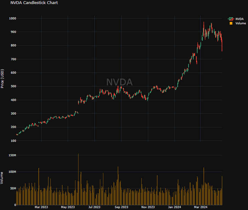
- Plotting the AMD candlesticks vs volume Plotly chart
# Plotting candlestick chart without indicators
from plotly.subplots import make_subplots
import plotly.graph_objects as go
start='2023-01-01'
# Downloading Apple Stocks
nvda = yf.download('AMD', start = start)

fig = make_subplots(rows=2, cols=1, shared_xaxes=True, vertical_spacing=0.05, row_heights = [0.7, 0.3])
fig.add_trace(go.Candlestick(x=nvda.index,
                             open=nvda['Open'],
                             high=nvda['High'],
                             low=nvda['Low'],
                             close=nvda['Adj Close'],
                             name='AMD'),
              row=1, col=1)


# Plotting volume chart on the second row
fig.add_trace(go.Bar(x=nvda.index,
                     y=nvda['Volume'],
                     name='Volume',
                     marker=dict(color='orange', opacity=1.0)),
              row=2, col=1)

# Plotting annotation
fig.add_annotation(text='AMD',
                    font=dict(color='white', size=40),
                    xref='paper', yref='paper',
                    x=0.5, y=0.65,
                    showarrow=False,
                    opacity=0.2)

# Configuring layout
fig.update_layout(title='AMD Candlestick Chart',
                  yaxis=dict(title='Price (USD)'),
                  height=1000,
                 template = 'plotly_dark')

# Configuring axes and subplots
fig.update_xaxes(rangeslider_visible=False, row=1, col=1)
fig.update_xaxes(rangeslider_visible=False, row=2, col=1)
fig.update_yaxes(title_text='Price (USD)', row=1, col=1)
fig.update_yaxes(title_text='Volume', row=2, col=1)

fig.show()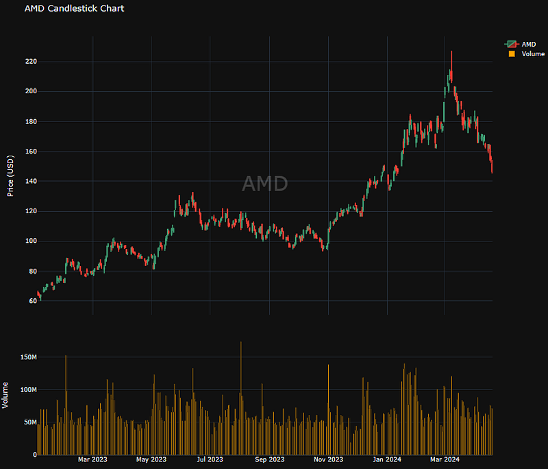
- Plotting the MSI candlesticks vs volume Plotly chart
# Plotting candlestick chart without indicators
from plotly.subplots import make_subplots
import plotly.graph_objects as go
start='2023-01-01'
# Downloading Apple Stocks
nvda = yf.download('MSI', start = start)

fig = make_subplots(rows=2, cols=1, shared_xaxes=True, vertical_spacing=0.05, row_heights = [0.7, 0.3])
fig.add_trace(go.Candlestick(x=nvda.index,
                             open=nvda['Open'],
                             high=nvda['High'],
                             low=nvda['Low'],
                             close=nvda['Adj Close'],
                             name='MSI'),
              row=1, col=1)


# Plotting volume chart on the second row
fig.add_trace(go.Bar(x=nvda.index,
                     y=nvda['Volume'],
                     name='Volume',
                     marker=dict(color='orange', opacity=1.0)),
              row=2, col=1)

# Plotting annotation
fig.add_annotation(text='MSI',
                    font=dict(color='white', size=40),
                    xref='paper', yref='paper',
                    x=0.5, y=0.65,
                    showarrow=False,
                    opacity=0.2)

# Configuring layout
fig.update_layout(title='MSI Candlestick Chart',
                  yaxis=dict(title='Price (USD)'),
                  height=1000,
                 template = 'plotly_dark')

# Configuring axes and subplots
fig.update_xaxes(rangeslider_visible=False, row=1, col=1)
fig.update_xaxes(rangeslider_visible=False, row=2, col=1)
fig.update_yaxes(title_text='Price (USD)', row=1, col=1)
fig.update_yaxes(title_text='Volume', row=2, col=1)

fig.show()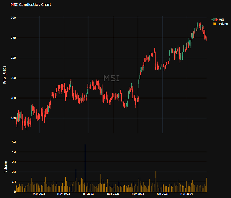
- Plotting the INTC candlesticks vs volume Plotly chart
# Plotting candlestick chart without indicators
from plotly.subplots import make_subplots
import plotly.graph_objects as go
start='2023-01-01'
# Downloading Apple Stocks
nvda = yf.download('INTC', start = start)

fig = make_subplots(rows=2, cols=1, shared_xaxes=True, vertical_spacing=0.05, row_heights = [0.7, 0.3])
fig.add_trace(go.Candlestick(x=nvda.index,
                             open=nvda['Open'],
                             high=nvda['High'],
                             low=nvda['Low'],
                             close=nvda['Adj Close'],
                             name='INTC'),
              row=1, col=1)


# Plotting volume chart on the second row
fig.add_trace(go.Bar(x=nvda.index,
                     y=nvda['Volume'],
                     name='Volume',
                     marker=dict(color='orange', opacity=1.0)),
              row=2, col=1)

# Plotting annotation
fig.add_annotation(text='INTC',
                    font=dict(color='white', size=40),
                    xref='paper', yref='paper',
                    x=0.5, y=0.65,
                    showarrow=False,
                    opacity=0.2)

# Configuring layout
fig.update_layout(title='INTC Candlestick Chart',
                  yaxis=dict(title='Price (USD)'),
                  height=1000,
                 template = 'plotly_dark')

# Configuring axes and subplots
fig.update_xaxes(rangeslider_visible=False, row=1, col=1)
fig.update_xaxes(rangeslider_visible=False, row=2, col=1)
fig.update_yaxes(title_text='Price (USD)', row=1, col=1)
fig.update_yaxes(title_text='Volume', row=2, col=1)

fig.show()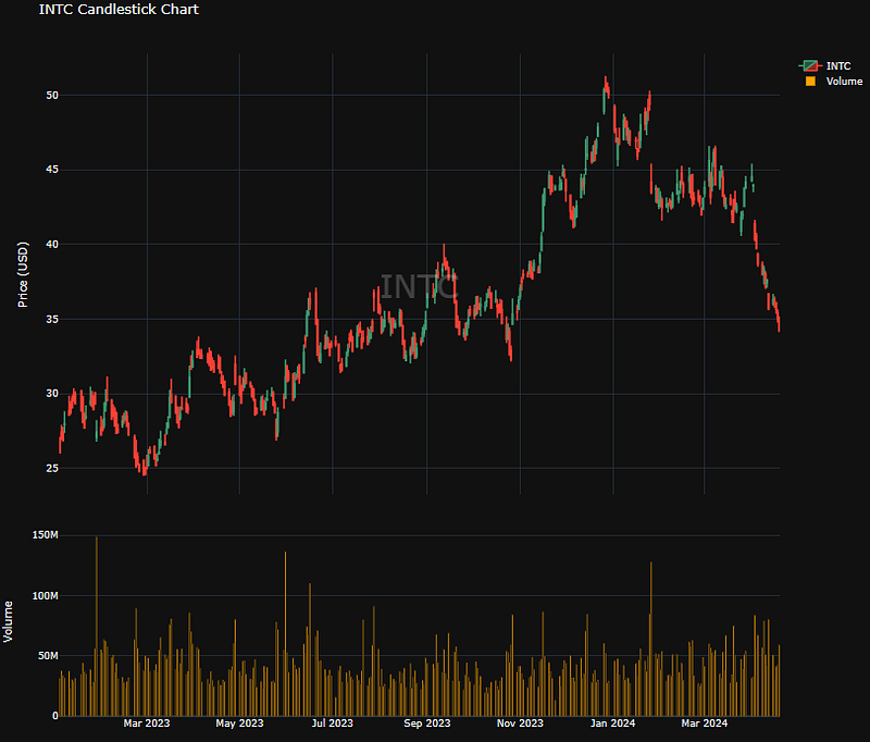
Descriptive Statistics
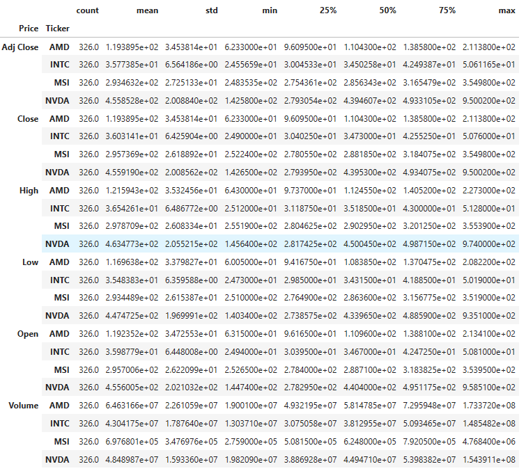
- Calculating aggregating statistics of the above stock data
data0.describe().T
- We can also split the summary statistics by considering 2Y period as an example:
nvda = yf.Ticker("NVDA").history(period='2y')['Close']
amd= yf.Ticker("AMD").history(period='2y')['Close']
msi= yf.Ticker("MSI").history(period='2y')['Close']
intc=yf.Ticker("INTC").history(period='2y')['Close']

#NVDA

print(nvda.mean())
print(nvda.median())
print(nvda.min())
print(nvda.max())
print(nvda.std())
print(nvda.mode())
nvda.describe()

351.51937653861984
274.44195556640625
112.18624114990234
950.02001953125
215.39582337067006
0    131.661697
1    132.511063
2    495.196777
Name: Close, dtype: float64
count    503.000000
mean     351.519377
std      215.395823
min      112.186241
25%      169.834717
50%      274.441956
75%      465.303574
max      950.020020
Name: Close, dtype: float64

#AMD

print(amd.mean())
print(amd.median())
print(amd.min())
print(amd.max())
print(amd.std())
print(amd.mode())
amd.describe()

105.61481091326795
98.01000213623047
55.939998626708984
211.3800048828125
34.499407320143966
0      75.250000
1      76.769997
2      84.639999
3      86.989998
4      89.839996
5     106.589996
6     115.820000
7     117.930000
8     138.580002
9     174.229996
10    178.699997
Name: Close, dtype: float64
count    503.000000
mean     105.614811
std       34.499407
min       55.939999
25%       81.500000
50%       98.010002
75%      117.845001
max      211.380005
Name: Close, dtype: float64

#MSI

print(msi.mean())
print(msi.median())
print(msi.min())
print(msi.max())
print(msi.std())
print(msi.mode())
msi.describe()

271.0420894736561
274.6322021484375
192.705078125
354.9800109863281
39.35118718826124
0    221.097916
1    252.675888
2    281.137085
3    281.982330
4    327.413727
Name: Close, dtype: float64
count    503.000000
mean     271.042089
std       39.351187
min      192.705078
25%      244.888878
50%      274.632202
75%      291.911865
max      354.980011
Name: Close, dtype: float64

#INTC

print(intc.mean())
print(intc.median())
print(intc.min())
print(intc.max())
print(intc.std())
print(intc.mode())
intc.describe()

34.70531823478684
34.16352462768555
24.0722599029541
50.61164855957031
6.538710173950736
0    25.927670
1    27.992682
Name: Close, dtype: float64
count    503.000000
mean      34.705318
std        6.538710
min       24.072260
25%       28.975665
50%       34.163525
75%       39.978010
max       50.611649
Name: Close, dtype: float64
Stock Returns, Volatility & Correlations
- Calculating stock returns, volatility and correlations
# Packages
import numpy as np
import pandas as pd
import matplotlib.pyplot as plt
%matplotlib inline

# Read Data
# Define the ticker list
import pandas as pd
tickers_list = ['NVDA', 'INTC', 'AMD', 'MSI']

# Fetch the data
import yfinance as yf
data = yf.download(tickers_list,'2023-1-1')['Adj Close']

# Print first 5 rows of the data
print(data.tail())
Ticker             AMD       INTC         MSI        NVDA
Date
2024-04-15  160.320007  36.310001  338.579987  860.010010
2024-04-16  163.460007  36.259998  340.109985  874.150024
2024-04-17  154.020004  35.680000  340.510010  840.349976
2024-04-18  155.080002  35.040001  339.459991  846.710022
2024-04-19  146.639999  34.200001  339.649994  762.000000
# Volatility of 4 stocks
data.pct_change().apply(lambda x: np.log(1+x)).std().apply(lambda x: x*np.sqrt(250)).plot(kind='bar')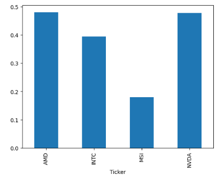
- Calculating covariance of log percentage change
# Log of percentage change cov
cov_matrix = data.pct_change().apply(lambda x: np.log(1+x)).cov()
cov_matrix

Ticker AMD    INTC     MSI      NVDA
Ticker
AMD 0.000925 0.000308 0.000072 0.000628
INTC 0.000308 0.000623 0.000054 0.000181
MSI 0.000072 0.000054 0.000130 0.000051
NVDA 0.000628 0.000181 0.000051 0.000913- Calculating correlations of log percentage change
corr_matrix = data.pct_change().apply(lambda x: np.log(1+x)).corr()
corr_matrix

Ticker AMD     INTC     MSI     NVDA
Ticker
AMD 1.000000 0.405428 0.207200 0.684001
INTC 0.405428 1.000000 0.189382 0.239388
MSI 0.207200 0.189382 1.000000 0.149202
NVDA 0.684001 0.239388 0.149202 1.000000- NVDA stock correlations
data['NVDA'].corr(data['AMD'])
0.9365483296876527
data['NVDA'].corr(data['MSI'])
0.9002879914460777
data['NVDA'].corr(data['INTC'])
0.73578743334689- Calculating annual std
# Volatility is given by the annual standard deviation. We multiply by 250 because there are 250 trading days/year.
ann_sd = data.pct_change().apply(lambda x: np.log(1+x)).std().apply(lambda x: x*np.sqrt(250))
ann_sd
Ticker
AMD     0.480784
INTC    0.394629
MSI     0.180365
NVDA    0.477675
dtype: float64- Calculating yearly returns
# Yearly returns for individual companies
ind_er = data.resample('YE').last().pct_change().mean()
ind_er
Ticker
AMD    -0.005224
INTC   -0.317408
MSI     0.087934
NVDA    0.538782
dtype: float64- Comparing yearly returns vs annual volatility
assets = pd.concat([ind_er, ann_sd], axis=1) # Creating a table for visualising returns and volatility of assets
assets.columns = ['Returns', 'Volatility']
assets

     Returns Volatility
Ticker
AMD -0.005224 0.480784
INTC -0.317408 0.394629
MSI 0.087934 0.180365
NVDA 0.538782 0.477675
Stock Returns vs Benchmark
- Adding the ^GSPC benchmark and calculating the 2Y stock returns by fetching the Adj Close price
import numpy as np # linear algebra
import pandas as pd # data processing, CSV file I/O (e.g. pd.read_csv)
import matplotlib.pyplot as plt
import plotly.express as px
import pandas_datareader as web
from datetime import datetime as dt, timedelta as td
end = dt.today()
start = end - td(days=2*365)

stocks = ['NVDA', 'INTC', 'AMD', 'MSI','^GSPC']

# Fetch the data
import yfinance as yf
df = yf.download(stocks,start=start,end=end)['Adj Close']

px.line(df * 100 / df.iloc[0])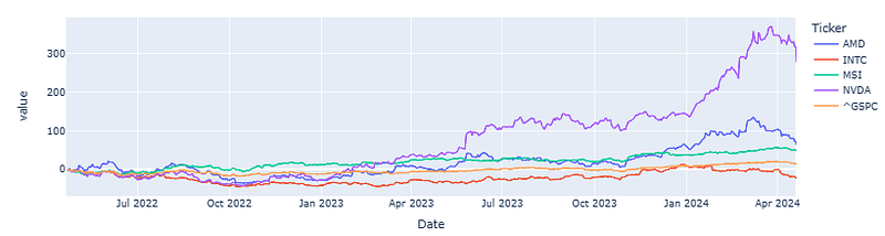
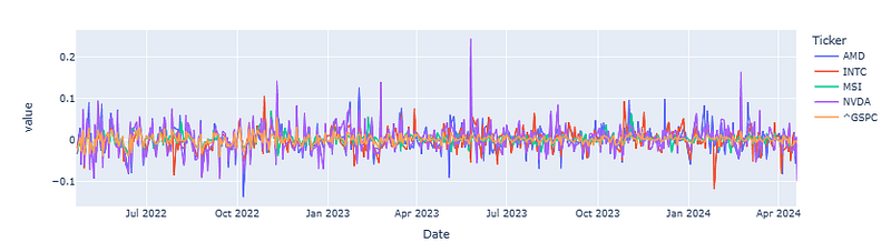
- Calculating the daily percentage change
ret_port = df.pct_change()
px.line(ret_port)
- Calculating the cumulative return
cumretport = (1 + ret_port).cumprod() - 1
px.line(cumretport*100)- Calculating the mean annual log return and beta
df_return = np.log(df / df.shift())
(df_return.mean() * 12).plot.bar()
plt.title(f'Annual log return')
cov = df_return.cov() * 12
market_cov = cov.iloc[0,1]
var_market = cov.iloc[1,1]
beta = market_cov / var_market
print (beta)
0.7333758533237972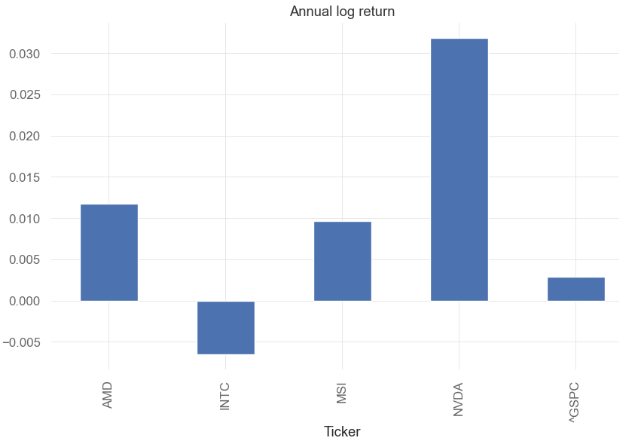
Stock Beta
- Calculating the 2Y stock beta
def get_beta(stock):
    start=dt.today() - td(days=365*2)
    df = yf.download([stock, '^GSPC'],start=start)['Adj Close']
    df_return = np.log(df / df.shift())
    (df_return.mean() * 12).plot.bar(title="Annual Log Return")
    cov = df_return.cov() * 12
    market_cov = cov.iloc[0,1]
    var_market = cov.iloc[1,1]
    beta = market_cov / var_market
    print(f'Beta 2Y of {stock.upper()} is : {beta}')
    return beta

get_beta('AMD')
1.9991308370043679

get_beta('MSI')
0.8368949323588019

get_beta('NVDA')
2.115183761971741

get_beta('INTC')
1.281878079502145
Sharpe Ratio
- Calculating the 2Y stock Sharpe ratio
def get_sharpe(stock):
    start=dt.today()-td(365*2)
    df = yf.download(stock,start=start)['Adj Close']

    ret = df.pct_change()

    ri = ret.mean()

    rf = (.025 / 365) # as we are making it daily. Since interest accrues on weekend we did 365

    sigma = ret.std()

    sr = (ri - rf) * 250 ** .5 / sigma # annualize the sharpe ratio

    print(f'Sharpe Ratio of {stock.upper()} is : {sr}')
    return sr

get_sharpe('AMD')
Sharpe Ratio of AMD is : 0.6789019155264734

get_sharpe('NVDA')
Sharpe Ratio of NVDA is : 1.477564006585132

get_sharpe('MSI')
Sharpe Ratio of MSI is : 0.9070020467720372

get_sharpe('INTC')
Sharpe Ratio of INTC is : -0.15157724728913474- We can compare these values against the quantstats.stats estimates, viz.
# Calculating Sharpe ratio
print('\n')
print("Sharpe Ratio for ^GSPC: ", qs.stats.sharpe(df['^GSPC']).round(2))
print('\n')
print("Sharpe Ratio for NVDA: ", qs.stats.sharpe(df['NVDA']).round(2))
print('\n')
print("Sharpe Ratio for AMD: ", qs.stats.sharpe(df['AMD']).round(2))
print('\n')
print("Sharpe Ratio for INTC: ", qs.stats.sharpe(df['INTC']).round(2))
print('\n')
print("Sharpe Ratio for MSI: ", qs.stats.sharpe(df['MSI']).round(2))

Sharpe Ratio for ^GSPC:  0.43


Sharpe Ratio for NVDA:  1.52


Sharpe Ratio for AMD:  0.72


Sharpe Ratio for INTC:  -0.11


Sharpe Ratio for MSI:  0.98
Company Financial Performance
- Fetching the NVDA current market cap, annual financials, and cashflow
ticker = yf.Ticker('NVDA')
current_market_cap = ticker.info['marketCap']
print(current_market_cap)
ticker.financials
2104474992640
2024-01-31 2023-01-31 2022-01-31 2021-01-31
Tax Effect Of Unusual Items 0.0 -284130000.0 0.0 0.0
Tax Rate For Calcs 0.12 0.21 0.019 0.017
Normalized EBITDA 35583000000.0 7340000000.0 11351000000.0 5691000000.0
Total Unusual Items 0.0 -1353000000.0 0.0 0.0
Total Unusual Items Excluding Goodwill 0.0 -1353000000.0 0.0 0.0
Net Income From Continuing Operation Net Minority Interest 29760000000.0 4368000000.0 9752000000.0 4332000000.0
Reconciled Depreciation 1508000000.0 1544000000.0 1174000000.0 1098000000.0
Reconciled Cost Of Revenue 16621000000.0 11618000000.0 9439000000.0 6279000000.0
EBITDA 35583000000.0 5987000000.0 11351000000.0 5691000000.0
EBIT 34075000000.0 4443000000.0 10177000000.0 4593000000.0
Net Interest Income 609000000.0 5000000.0 -207000000.0 -127000000.0
Interest Expense 257000000.0 262000000.0 236000000.0 184000000.0
Interest Income 866000000.0 267000000.0 29000000.0 57000000.0
Normalized Income 29760000000.0 5436870000.0 9752000000.0 4332000000.0
Net Income From Continuing And Discontinued Operation 29760000000.0 4368000000.0 9752000000.0 4332000000.0
Total Expenses 27950000000.0 21397000000.0 16873000000.0 12143000000.0
Total Operating Income As Reported 32972000000.0 4224000000.0 10041000000.0 4532000000.0
Diluted Average Shares 2494000000.0 2507000000.0 2535000000.0 2512000000.0
Basic Average Shares 2469000000.0 2487000000.0 2496000000.0 2468000000.0
Diluted EPS 11.93 1.74 3.85 1.725
Basic EPS 12.05 1.76 3.91 1.755
Diluted NI Availto Com Stockholders 29760000000.0 4368000000.0 9752000000.0 4332000000.0
Net Income Common Stockholders 29760000000.0 4368000000.0 9752000000.0 4332000000.0
Net Income 29760000000.0 4368000000.0 9752000000.0 4332000000.0
Net Income Including Noncontrolling Interests 29760000000.0 4368000000.0 9752000000.0 4332000000.0
Net Income Continuous Operations 29760000000.0 4368000000.0 9752000000.0 4332000000.0
Tax Provision 4058000000.0 -187000000.0 189000000.0 77000000.0
Pretax Income 33818000000.0 4181000000.0 9941000000.0 4409000000.0
Other Income Expense 237000000.0 -1401000000.0 107000000.0 4000000.0
Other Non Operating Income Expenses 237000000.0 -48000000.0 107000000.0 4000000.0
Special Income Charges 0.0 -1353000000.0 0.0 0.0
Restructuring And Mergern Acquisition 0.0 1353000000.0 0.0 0.0
Net Non Operating Interest Income Expense 609000000.0 5000000.0 -207000000.0 -127000000.0
Interest Expense Non Operating 257000000.0 262000000.0 236000000.0 184000000.0
Interest Income Non Operating 866000000.0 267000000.0 29000000.0 57000000.0
Operating Income 32972000000.0 5577000000.0 10041000000.0 4532000000.0
Operating Expense 11329000000.0 9779000000.0 7434000000.0 5864000000.0
Research And Development 8675000000.0 7339000000.0 5268000000.0 3924000000.0
Selling General And Administration 2654000000.0 2440000000.0 2166000000.0 1940000000.0
Gross Profit 44301000000.0 15356000000.0 17475000000.0 10396000000.0
Cost Of Revenue 16621000000.0 11618000000.0 9439000000.0 6279000000.0
Total Revenue 60922000000.0 26974000000.0 26914000000.0 16675000000.0
Operating Revenue 60922000000.0 26974000000.0 26914000000.0 16675000000.0
ticker.cashflow
2024-01-31 2023-01-31 2022-01-31 2021-01-31
Free Cash Flow 27021000000.0 3808000000.0 8132000000.0 4694000000.0
Repurchase Of Capital Stock -9533000000.0 -10039000000.0 0.0 0.0
Repayment Of Debt -1250000000.0 0.0 -1000000000.0 0.0
Issuance Of Debt 0.0 0.0 4977000000.0 4968000000.0
Capital Expenditure -1069000000.0 -1833000000.0 -976000000.0 -1128000000.0
Interest Paid Supplemental Data 252000000.0 254000000.0 246000000.0 138000000.0
Income Tax Paid Supplemental Data 6549000000.0 1404000000.0 396000000.0 249000000.0
End Cash Position 7280000000.0 3389000000.0 1990000000.0 847000000.0
Beginning Cash Position 3389000000.0 1990000000.0 847000000.0 10896000000.0
Changes In Cash 3891000000.0 1399000000.0 1143000000.0 -10049000000.0
Financing Cash Flow -13633000000.0 -11617000000.0 1865000000.0 3804000000.0
Cash Flow From Continuing Financing Activities -13633000000.0 -11617000000.0 1865000000.0 3804000000.0
Net Other Financing Charges -2858000000.0 -1535000000.0 -1994000000.0 -963000000.0
Proceeds From Stock Option Exercised 403000000.0 355000000.0 281000000.0 194000000.0
Cash Dividends Paid -395000000.0 -398000000.0 -399000000.0 -395000000.0
Common Stock Dividend Paid NaN -398000000.0 -399000000.0 -395000000.0
Net Common Stock Issuance -9533000000.0 -10039000000.0 0.0 0.0
Common Stock Payments -9533000000.0 -10039000000.0 0.0 0.0
Net Issuance Payments Of Debt -1250000000.0 0.0 3977000000.0 4968000000.0
Net Long Term Debt Issuance -1250000000.0 0.0 3977000000.0 4968000000.0
Long Term Debt Payments -1250000000.0 0.0 -1000000000.0 0.0
Long Term Debt Issuance 0.0 0.0 4977000000.0 4968000000.0
Investing Cash Flow -10566000000.0 7375000000.0 -9830000000.0 -19675000000.0
Cash Flow From Continuing Investing Activities -10566000000.0 7375000000.0 -9830000000.0 -19675000000.0
Net Investment Purchase And Sale -9414000000.0 9257000000.0 -8591000000.0 -10023000000.0
Sale Of Investment 9782000000.0 21231000000.0 16220000000.0 9319000000.0
Purchase Of Investment -19196000000.0 -11974000000.0 -24811000000.0 -19342000000.0
Net Business Purchase And Sale -83000000.0 -49000000.0 -263000000.0 -8524000000.0
Purchase Of Business -83000000.0 -49000000.0 -263000000.0 -8524000000.0
Net PPE Purchase And Sale -1069000000.0 -1833000000.0 -976000000.0 -1128000000.0
Purchase Of PPE -1069000000.0 -1833000000.0 -976000000.0 -1128000000.0
Capital Expenditure Reported NaN NaN NaN -1128000000.0
Operating Cash Flow 28090000000.0 5641000000.0 9108000000.0 5822000000.0
Cash Flow From Continuing Operating Activities 28090000000.0 5641000000.0 9108000000.0 5822000000.0
Change In Working Capital -3722000000.0 -2207000000.0 -3363000000.0 -703000000.0
Change In Other Working Capital NaN NaN NaN 163000000.0
Change In Other Current Liabilities 514000000.0 252000000.0 192000000.0 163000000.0
Change In Payables And Accrued Expense 3556000000.0 790000000.0 1149000000.0 602000000.0
Change In Accrued Expense 2025000000.0 1341000000.0 581000000.0 290000000.0
Change In Payable 1531000000.0 -551000000.0 568000000.0 312000000.0
Change In Account Payable 1531000000.0 -551000000.0 568000000.0 312000000.0
Change In Prepaid Assets -1522000000.0 -1517000000.0 -1715000000.0 -394000000.0
Change In Inventory -98000000.0 -2554000000.0 -774000000.0 -524000000.0
Change In Receivables -6172000000.0 822000000.0 -2215000000.0 -550000000.0
Changes In Account Receivables -6172000000.0 822000000.0 -2215000000.0 -550000000.0
Other Non Cash Items -278000000.0 1346000000.0 47000000.0 -20000000.0
Stock Based Compensation 3549000000.0 2709000000.0 2004000000.0 1397000000.0
Deferred Tax -2489000000.0 -2164000000.0 -406000000.0 -282000000.0
Deferred Income Tax -2489000000.0 -2164000000.0 -406000000.0 -282000000.0
Depreciation Amortization Depletion 1508000000.0 1544000000.0 1174000000.0 1098000000.0
Depreciation And Amortization 1508000000.0 1544000000.0 1174000000.0 1098000000.0
Operating Gains Losses -238000000.0 45000000.0 -100000000.0 NaN
Gain Loss On Investment Securities -238000000.0 45000000.0 -100000000.0 NaN
Net Income From Continuing Operations 29760000000.0 4368000000.0 9752000000.0 4332000000.0- Fetching the AMD current market cap, annual financials, and cashflow
ticker = yf.Ticker('AMD')
current_market_cap = ticker.info['marketCap']
print(current_market_cap)
ticker.financials
248319901696

2023-12-31 2022-12-31 2021-12-31 2020-12-31
Tax Effect Of Unusual Items 0.0 0.0 -978740.801308 -14580000.0
Tax Rate For Calcs 0.21 0.21 0.13982 0.27
Normalized EBITDA 4149000000.0 5534000000.0 4173000000.0 1730000000.0
Total Unusual Items 0.0 0.0 -7000000.0 -54000000.0
Total Unusual Items Excluding Goodwill 0.0 0.0 -7000000.0 -54000000.0
Net Income From Continuing Operation Net Minority Interest 854000000.0 1320000000.0 3162000000.0 2490000000.0
Reconciled Depreciation 3551000000.0 4262000000.0 463000000.0 354000000.0
Reconciled Cost Of Revenue 10538000000.0 10836000000.0 8042000000.0 5062000000.0
EBITDA 4149000000.0 5534000000.0 4166000000.0 1676000000.0
EBIT 598000000.0 1272000000.0 3703000000.0 1322000000.0
Net Interest Income 100000000.0 -23000000.0 -26000000.0 -39000000.0
Interest Expense 106000000.0 88000000.0 34000000.0 47000000.0
Interest Income 206000000.0 65000000.0 8000000.0 8000000.0
Normalized Income 854000000.0 1320000000.0 3168021259.198692 2529420000.0
Net Income From Continuing And Discontinued Operation 854000000.0 1320000000.0 3162000000.0 2490000000.0
Total Expenses 22279000000.0 22337000000.0 12786000000.0 8394000000.0
Total Operating Income As Reported 401000000.0 1264000000.0 3648000000.0 1369000000.0
Diluted Average Shares 1625000000.0 1571000000.0 1229000000.0 1207000000.0
Basic Average Shares 1614000000.0 1561000000.0 1213000000.0 1184000000.0
Diluted EPS 0.53 0.84 2.57 2.06
Basic EPS 0.53 0.85 2.61 2.1
Diluted NI Availto Com Stockholders 854000000.0 1320000000.0 3162000000.0 2491000000.0
Average Dilution Earnings NaN 0.0 0.0 1000000.0
Net Income Common Stockholders 854000000.0 1320000000.0 3162000000.0 2490000000.0
Net Income 854000000.0 1320000000.0 3162000000.0 2490000000.0
Net Income Including Noncontrolling Interests 854000000.0 1320000000.0 3162000000.0 2490000000.0
Net Income Continuous Operations 854000000.0 1320000000.0 3162000000.0 2490000000.0
Earnings From Equity Interest Net Of Tax 16000000.0 14000000.0 6000000.0 5000000.0
Tax Provision -346000000.0 -122000000.0 513000000.0 -1210000000.0
Pretax Income 492000000.0 1184000000.0 3669000000.0 1275000000.0
Other Income Expense -9000000.0 -57000000.0 47000000.0 -55000000.0
Other Non Operating Income Expenses -8000000.0 5000000.0 -2000000.0 -3000000.0
Special Income Charges 0.0 0.0 -7000000.0 -54000000.0
Other Special Charges NaN NaN 7000000.0 54000000.0
Earnings From Equity Interest -1000000.0 -62000000.0 56000000.0 2000000.0
Net Non Operating Interest Income Expense 100000000.0 -23000000.0 -26000000.0 -39000000.0
Interest Expense Non Operating 106000000.0 88000000.0 34000000.0 47000000.0
Interest Income Non Operating 206000000.0 65000000.0 8000000.0 8000000.0
Operating Income 401000000.0 1264000000.0 3648000000.0 1369000000.0
Operating Expense 10059000000.0 9339000000.0 4281000000.0 2978000000.0
Other Operating Expenses -34000000.0 -102000000.0 -12000000.0 NaN
Depreciation Amortization Depletion Income Statement 1869000000.0 2100000000.0 0.0 0.0
Depreciation And Amortization In Income Statement 1869000000.0 2100000000.0 0.0 0.0
Amortization 1869000000.0 2100000000.0 0.0 0.0
Amortization Of Intangibles Income Statement 1869000000.0 2100000000.0 0.0 0.0
Research And Development 5872000000.0 5005000000.0 2845000000.0 1983000000.0
Selling General And Administration 2352000000.0 2336000000.0 1448000000.0 995000000.0
Gross Profit 10460000000.0 10603000000.0 7929000000.0 4347000000.0
Cost Of Revenue 12220000000.0 12998000000.0 8505000000.0 5416000000.0
Total Revenue 22680000000.0 23601000000.0 16434000000.0 9763000000.0
Operating Revenue 22680000000.0 23601000000.0 16434000000.0 9763000000.0
ticker.cashflow
2023-12-31 2022-12-31 2021-12-31 2020-12-31
Free Cash Flow 1121000000.0 3115000000.0 3220000000.0 777000000.0
Repurchase Of Capital Stock -1412000000.0 -4108000000.0 -1999000000.0 -78000000.0
Repayment Of Debt 0.0 -312000000.0 0.0 -200000000.0
Issuance Of Debt 0.0 991000000.0 0.0 200000000.0
Capital Expenditure -546000000.0 -450000000.0 -301000000.0 -294000000.0
Interest Paid Supplemental Data 84000000.0 85000000.0 25000000.0 31000000.0
Income Tax Paid Supplemental Data 523000000.0 685000000.0 35000000.0 8000000.0
End Cash Position 3933000000.0 4835000000.0 2535000000.0 1595000000.0
Beginning Cash Position 4835000000.0 2535000000.0 1595000000.0 1470000000.0
Changes In Cash -902000000.0 2300000000.0 940000000.0 125000000.0
Financing Cash Flow -1146000000.0 -3264000000.0 -1895000000.0 6000000.0
Cash Flow From Continuing Financing Activities -1146000000.0 -3264000000.0 -1895000000.0 6000000.0
Net Other Financing Charges -2000000.0 -2000000.0 NaN -1000000.0
Proceeds From Stock Option Exercised 268000000.0 167000000.0 104000000.0 85000000.0
Net Common Stock Issuance -1412000000.0 -4108000000.0 -1999000000.0 -78000000.0
Common Stock Payments -1412000000.0 -4108000000.0 -1999000000.0 -78000000.0
Net Issuance Payments Of Debt 0.0 679000000.0 0.0 0.0
Net Short Term Debt Issuance NaN NaN 0.0 200000000.0
Short Term Debt Issuance NaN NaN 0.0 200000000.0
Net Long Term Debt Issuance 0.0 679000000.0 0.0 0.0
Long Term Debt Payments 0.0 -312000000.0 0.0 -200000000.0
Long Term Debt Issuance 0.0 991000000.0 0.0 200000000.0
Investing Cash Flow -1423000000.0 1999000000.0 -686000000.0 -952000000.0
Cash Flow From Continuing Investing Activities -1423000000.0 1999000000.0 -686000000.0 -952000000.0
Net Other Investing Changes -11000000.0 -16000000.0 -7000000.0 NaN
Net Investment Purchase And Sale -735000000.0 1643000000.0 -378000000.0 -658000000.0
Sale Of Investment 2987000000.0 4310000000.0 1678000000.0 192000000.0
Purchase Of Investment -3722000000.0 -2667000000.0 -2056000000.0 -850000000.0
Net Business Purchase And Sale -131000000.0 822000000.0 0.0 0.0
Sale Of Business 0.0 2366000000.0 0.0 0.0
Purchase Of Business -131000000.0 -1544000000.0 0.0 0.0
Net PPE Purchase And Sale -546000000.0 -450000000.0 -301000000.0 -294000000.0
Purchase Of PPE -546000000.0 -450000000.0 -301000000.0 -294000000.0
Operating Cash Flow 1667000000.0 3565000000.0 3521000000.0 1071000000.0
Cash Flow From Continuing Operating Activities 1667000000.0 3565000000.0 3521000000.0 1071000000.0
Change In Working Capital -3049000000.0 -1846000000.0 -774000000.0 -931000000.0
Change In Payables And Accrued Expense -740000000.0 1856000000.0 1334000000.0 -74000000.0
Change In Accrued Expense -221000000.0 546000000.0 526000000.0 574000000.0
Change In Payable -519000000.0 1310000000.0 808000000.0 -648000000.0
Change In Account Payable -419000000.0 931000000.0 801000000.0 -513000000.0
Change In Prepaid Assets -472000000.0 -1197000000.0 -920000000.0 -231000000.0
Change In Inventory -580000000.0 -1401000000.0 -556000000.0 -417000000.0
Change In Receivables -1257000000.0 -1104000000.0 -632000000.0 -209000000.0
Changes In Account Receivables -1250000000.0 -1091000000.0 -640000000.0 -219000000.0
Other Non Cash Items -64000000.0 175000000.0 -2000000.0 22000000.0
Stock Based Compensation 1384000000.0 1081000000.0 379000000.0 274000000.0
Asset Impairment Charge NaN NaN NaN 0.0
Deferred Tax -1019000000.0 -1505000000.0 308000000.0 -1223000000.0
Deferred Income Tax -1019000000.0 -1505000000.0 308000000.0 -1223000000.0
Depreciation Amortization Depletion 3551000000.0 4262000000.0 463000000.0 354000000.0
Depreciation And Amortization 3551000000.0 4262000000.0 463000000.0 354000000.0
Depreciation 3551000000.0 4262000000.0 463000000.0 354000000.0
Operating Gains Losses 10000000.0 78000000.0 -15000000.0 85000000.0
Earnings Losses From Equity Investments -1000000.0 62000000.0 -56000000.0 -2000000.0
Gain Loss On Investment Securities NaN 62000000.0 -56000000.0 -2000000.0
Gain Loss On Sale Of PPE 11000000.0 16000000.0 34000000.0 33000000.0
Net Income From Continuing Operations 854000000.0 1320000000.0 3162000000.0 2490000000.0- Fetching the MSI current market cap, annual financials, and cashflow
ticker = yf.Ticker('MSI')
current_market_cap = ticker.info['marketCap']
print(current_market_cap)
ticker.financials

56290332672

2023-12-31 2022-12-31 2021-12-31 2020-12-31
Tax Effect Of Unusual Items -20502000.0 -14014000.0 -17550000.0 -19740000.0
Tax Rate For Calcs 0.201 0.098 0.195 0.188
Normalized EBITDA 2853000000.0 2338000000.0 2295000000.0 1921000000.0
Total Unusual Items -102000000.0 -143000000.0 -90000000.0 -105000000.0
Total Unusual Items Excluding Goodwill -102000000.0 -143000000.0 -90000000.0 -105000000.0
Net Income From Continuing Operation Net Minority Interest 1709000000.0 1363000000.0 1245000000.0 949000000.0
Reconciled Depreciation 356000000.0 440000000.0 438000000.0 409000000.0
Reconciled Cost Of Revenue 4829000000.0 4700000000.0 3929000000.0 3612000000.0
EBITDA 2751000000.0 2195000000.0 2205000000.0 1816000000.0
EBIT 2395000000.0 1755000000.0 1767000000.0 1407000000.0
Net Interest Income -216000000.0 -226000000.0 -208000000.0 -220000000.0
Interest Expense 249000000.0 240000000.0 215000000.0 233000000.0
Interest Income 33000000.0 14000000.0 7000000.0 13000000.0
Normalized Income 1790498000.0 1491986000.0 1317450000.0 1034260000.0
Net Income From Continuing And Discontinued Operation 1709000000.0 1363000000.0 1245000000.0 949000000.0
Total Expenses 7520000000.0 7246000000.0 6331000000.0 5919000000.0
Total Operating Income As Reported 2294000000.0 1661000000.0 1667000000.0 1383000000.0
Diluted Average Shares NaN 171900000.0 173600000.0 174100000.0
Basic Average Shares NaN 167500000.0 169200000.0 170000000.0
Diluted EPS NaN 7.93 7.17 5.45
Basic EPS NaN 8.14 7.36 5.58
Diluted NI Availto Com Stockholders 1709000000.0 1363000000.0 1245000000.0 949000000.0
Net Income Common Stockholders 1709000000.0 1363000000.0 1245000000.0 949000000.0
Net Income 1709000000.0 1363000000.0 1245000000.0 949000000.0
Minority Interests -5000000.0 -4000000.0 -5000000.0 -4000000.0
Net Income Including Noncontrolling Interests 1714000000.0 1367000000.0 1250000000.0 953000000.0
Net Income Continuous Operations 1714000000.0 1367000000.0 1250000000.0 953000000.0
Tax Provision 432000000.0 148000000.0 302000000.0 221000000.0
Pretax Income 2146000000.0 1515000000.0 1552000000.0 1174000000.0
Other Income Expense -96000000.0 -125000000.0 -80000000.0 -101000000.0
Other Non Operating Income Expenses 6000000.0 123000000.0 5000000.0 1000000.0
Special Income Charges -82000000.0 -92000000.0 -70000000.0 -90000000.0
Gain On Sale Of Ppe NaN 0.0 0.0 50000000.0
Gain On Sale Of Business -24000000.0 0.0 0.0 NaN
Other Special Charges 4000000.0 14000000.0 21000000.0 65000000.0
Write Off 16000000.0 1000000.0 0.0 9000000.0
Impairment Of Capital Assets 9000000.0 36000000.0 10000000.0 0.0
Restructuring And Mergern Acquisition 29000000.0 41000000.0 39000000.0 66000000.0
Earnings From Equity Interest 0.0 18000000.0 5000000.0 3000000.0
Gain On Sale Of Security -20000000.0 -51000000.0 -20000000.0 -15000000.0
Net Non Operating Interest Income Expense -216000000.0 -226000000.0 -208000000.0 -220000000.0
Interest Expense Non Operating 249000000.0 240000000.0 215000000.0 233000000.0
Interest Income Non Operating 33000000.0 14000000.0 7000000.0 13000000.0
Operating Income 2458000000.0 1866000000.0 1840000000.0 1495000000.0
Operating Expense 2512000000.0 2363000000.0 2200000000.0 2113000000.0
Other Operating Expenses 15000000.0 NaN NaN NaN
Depreciation Amortization Depletion Income Statement 177000000.0 257000000.0 236000000.0 215000000.0
Depreciation And Amortization In Income Statement 177000000.0 257000000.0 236000000.0 215000000.0
Amortization 177000000.0 257000000.0 236000000.0 215000000.0
Amortization Of Intangibles Income Statement 177000000.0 257000000.0 236000000.0 215000000.0
Research And Development 858000000.0 779000000.0 734000000.0 686000000.0
Selling General And Administration 1462000000.0 1327000000.0 1230000000.0 1212000000.0
General And Administrative Expense 1462000000.0 1327000000.0 1230000000.0 1212000000.0
Other Gand A 1561000000.0 1450000000.0 1353000000.0 1293000000.0
Salaries And Wages -99000000.0 -123000000.0 -123000000.0 -81000000.0
Gross Profit 4970000000.0 4229000000.0 4040000000.0 3608000000.0
Cost Of Revenue 5008000000.0 4883000000.0 4131000000.0 3806000000.0
Total Revenue 9978000000.0 9112000000.0 8171000000.0 7414000000.0
Operating Revenue 9978000000.0 9112000000.0 8171000000.0 7414000000.0
ticker.cashflow
2023-12-31 2022-12-31 2021-12-31 2020-12-31
Free Cash Flow 1791000000.0 1567000000.0 1594000000.0 1396000000.0
Repurchase Of Capital Stock -804000000.0 -836000000.0 -528000000.0 -612000000.0
Repayment Of Debt -1000000.0 -285000000.0 -353000000.0 -1714000000.0
Issuance Of Debt 0.0 595000000.0 844000000.0 1692000000.0
Issuance Of Capital Stock 104000000.0 156000000.0 102000000.0 108000000.0
Capital Expenditure -253000000.0 -256000000.0 -243000000.0 -217000000.0
Interest Paid Supplemental Data 234000000.0 226000000.0 207000000.0 217000000.0
Income Tax Paid Supplemental Data 587000000.0 307000000.0 257000000.0 181000000.0
End Cash Position 1705000000.0 1325000000.0 1874000000.0 1254000000.0
Beginning Cash Position 1325000000.0 1874000000.0 1254000000.0 1001000000.0
Effect Of Exchange Rate Changes 45000000.0 -79000000.0 -46000000.0 43000000.0
Changes In Cash 335000000.0 -470000000.0 666000000.0 210000000.0
Financing Cash Flow -1295000000.0 -906000000.0 -429000000.0 -966000000.0
Cash Flow From Continuing Financing Activities -1295000000.0 -906000000.0 -429000000.0 -966000000.0
Net Other Financing Charges -5000000.0 -6000000.0 -12000000.0 -4000000.0
Cash Dividends Paid -589000000.0 -530000000.0 -482000000.0 -436000000.0
Common Stock Dividend Paid -589000000.0 -530000000.0 -482000000.0 -436000000.0
Net Common Stock Issuance -700000000.0 -680000000.0 -426000000.0 -504000000.0
Common Stock Payments -804000000.0 -836000000.0 -528000000.0 -612000000.0
Common Stock Issuance 104000000.0 156000000.0 102000000.0 108000000.0
Net Issuance Payments Of Debt -1000000.0 310000000.0 491000000.0 -22000000.0
Net Short Term Debt Issuance NaN 0.0 0.0 0.0
Short Term Debt Payments NaN 0.0 0.0 -800000000.0
Short Term Debt Issuance NaN 0.0 0.0 800000000.0
Net Long Term Debt Issuance -1000000.0 310000000.0 491000000.0 -22000000.0
Long Term Debt Payments -1000000.0 -285000000.0 -353000000.0 -914000000.0
Long Term Debt Issuance 0.0 595000000.0 844000000.0 892000000.0
Investing Cash Flow -414000000.0 -1387000000.0 -742000000.0 -437000000.0
Cash Flow From Continuing Investing Activities -414000000.0 -1387000000.0 -742000000.0 -437000000.0
Net Investment Purchase And Sale 19000000.0 46000000.0 16000000.0 11000000.0
Sale Of Investment 19000000.0 46000000.0 16000000.0 11000000.0
Net Business Purchase And Sale -180000000.0 -1177000000.0 -521000000.0 -287000000.0
Purchase Of Business -180000000.0 -1177000000.0 -521000000.0 -287000000.0
Net PPE Purchase And Sale 0.0 0.0 6000000.0 56000000.0
Sale Of PPE 0.0 0.0 6000000.0 56000000.0
Capital Expenditure Reported -253000000.0 -256000000.0 -243000000.0 -217000000.0
Operating Cash Flow 2044000000.0 1823000000.0 1837000000.0 1613000000.0
Cash Flow From Continuing Operating Activities 2044000000.0 1823000000.0 1837000000.0 1613000000.0
Change In Working Capital -276000000.0 -329000000.0 0.0 102000000.0
Change In Other Working Capital -70000000.0 -425000000.0 -92000000.0 -25000000.0
Change In Other Current Assets -82000000.0 -1000000.0 -205000000.0 167000000.0
Change In Payables And Accrued Expense -144000000.0 451000000.0 578000000.0 -116000000.0
Change In Payable -144000000.0 451000000.0 578000000.0 -116000000.0
Change In Account Payable -144000000.0 451000000.0 578000000.0 -116000000.0
Change In Inventory 200000000.0 -242000000.0 -284000000.0 -14000000.0
Change In Receivables -180000000.0 -112000000.0 3000000.0 90000000.0
Changes In Account Receivables -180000000.0 -112000000.0 3000000.0 90000000.0
Other Non Cash Items 38000000.0 23000000.0 3000000.0 -13000000.0
Stock Based Compensation 212000000.0 172000000.0 129000000.0 129000000.0
Asset Impairment Charge 0.0 147000000.0 0.0 NaN
Deferred Tax NaN NaN 34000000.0 -25000000.0
Deferred Income Tax NaN NaN 34000000.0 -25000000.0
Depreciation Amortization Depletion 356000000.0 440000000.0 438000000.0 409000000.0
Depreciation And Amortization 356000000.0 440000000.0 438000000.0 409000000.0
Operating Gains Losses NaN 3000000.0 17000000.0 58000000.0
Pension And Employee Benefit Expense NaN NaN 0.0 0.0
Gain Loss On Investment Securities NaN -3000000.0 -1000000.0 2000000.0
Net Income From Continuing Operations 1714000000.0 1367000000.0 1250000000.0 953000000.0- Fetching the INTC current market cap, annual financials, and cashflow
ticker = yf.Ticker('INTC')
current_market_cap = ticker.info['marketCap']
print(current_market_cap)
149054291968

ticker.financials

2023-12-31 2022-12-31 2021-12-31 2020-12-31
Tax Effect Of Unusual Items -20502000.0 -14014000.0 -17550000.0 -19740000.0
Tax Rate For Calcs 0.201 0.098 0.195 0.188
Normalized EBITDA 2853000000.0 2338000000.0 2295000000.0 1921000000.0
Total Unusual Items -102000000.0 -143000000.0 -90000000.0 -105000000.0
Total Unusual Items Excluding Goodwill -102000000.0 -143000000.0 -90000000.0 -105000000.0
Net Income From Continuing Operation Net Minority Interest 1709000000.0 1363000000.0 1245000000.0 949000000.0
Reconciled Depreciation 356000000.0 440000000.0 438000000.0 409000000.0
Reconciled Cost Of Revenue 4829000000.0 4700000000.0 3929000000.0 3612000000.0
EBITDA 2751000000.0 2195000000.0 2205000000.0 1816000000.0
EBIT 2395000000.0 1755000000.0 1767000000.0 1407000000.0
Net Interest Income -216000000.0 -226000000.0 -208000000.0 -220000000.0
Interest Expense 249000000.0 240000000.0 215000000.0 233000000.0
Interest Income 33000000.0 14000000.0 7000000.0 13000000.0
Normalized Income 1790498000.0 1491986000.0 1317450000.0 1034260000.0
Net Income From Continuing And Discontinued Operation 1709000000.0 1363000000.0 1245000000.0 949000000.0
Total Expenses 7520000000.0 7246000000.0 6331000000.0 5919000000.0
Total Operating Income As Reported 2294000000.0 1661000000.0 1667000000.0 1383000000.0
Diluted Average Shares NaN 171900000.0 173600000.0 174100000.0
Basic Average Shares NaN 167500000.0 169200000.0 170000000.0
Diluted EPS NaN 7.93 7.17 5.45
Basic EPS NaN 8.14 7.36 5.58
Diluted NI Availto Com Stockholders 1709000000.0 1363000000.0 1245000000.0 949000000.0
Net Income Common Stockholders 1709000000.0 1363000000.0 1245000000.0 949000000.0
Net Income 1709000000.0 1363000000.0 1245000000.0 949000000.0
Minority Interests -5000000.0 -4000000.0 -5000000.0 -4000000.0
Net Income Including Noncontrolling Interests 1714000000.0 1367000000.0 1250000000.0 953000000.0
Net Income Continuous Operations 1714000000.0 1367000000.0 1250000000.0 953000000.0
Tax Provision 432000000.0 148000000.0 302000000.0 221000000.0
Pretax Income 2146000000.0 1515000000.0 1552000000.0 1174000000.0
Other Income Expense -96000000.0 -125000000.0 -80000000.0 -101000000.0
Other Non Operating Income Expenses 6000000.0 123000000.0 5000000.0 1000000.0
Special Income Charges -82000000.0 -92000000.0 -70000000.0 -90000000.0
Gain On Sale Of Ppe NaN 0.0 0.0 50000000.0
Gain On Sale Of Business -24000000.0 0.0 0.0 NaN
Other Special Charges 4000000.0 14000000.0 21000000.0 65000000.0
Write Off 16000000.0 1000000.0 0.0 9000000.0
Impairment Of Capital Assets 9000000.0 36000000.0 10000000.0 0.0
Restructuring And Mergern Acquisition 29000000.0 41000000.0 39000000.0 66000000.0
Earnings From Equity Interest 0.0 18000000.0 5000000.0 3000000.0
Gain On Sale Of Security -20000000.0 -51000000.0 -20000000.0 -15000000.0
Net Non Operating Interest Income Expense -216000000.0 -226000000.0 -208000000.0 -220000000.0
Interest Expense Non Operating 249000000.0 240000000.0 215000000.0 233000000.0
Interest Income Non Operating 33000000.0 14000000.0 7000000.0 13000000.0
Operating Income 2458000000.0 1866000000.0 1840000000.0 1495000000.0
Operating Expense 2512000000.0 2363000000.0 2200000000.0 2113000000.0
Other Operating Expenses 15000000.0 NaN NaN NaN
Depreciation Amortization Depletion Income Statement 177000000.0 257000000.0 236000000.0 215000000.0
Depreciation And Amortization In Income Statement 177000000.0 257000000.0 236000000.0 215000000.0
Amortization 177000000.0 257000000.0 236000000.0 215000000.0
Amortization Of Intangibles Income Statement 177000000.0 257000000.0 236000000.0 215000000.0
Research And Development 858000000.0 779000000.0 734000000.0 686000000.0
Selling General And Administration 1462000000.0 1327000000.0 1230000000.0 1212000000.0
General And Administrative Expense 1462000000.0 1327000000.0 1230000000.0 1212000000.0
Other Gand A 1561000000.0 1450000000.0 1353000000.0 1293000000.0
Salaries And Wages -99000000.0 -123000000.0 -123000000.0 -81000000.0
Gross Profit 4970000000.0 4229000000.0 4040000000.0 3608000000.0
Cost Of Revenue 5008000000.0 4883000000.0 4131000000.0 3806000000.0
Total Revenue 9978000000.0 9112000000.0 8171000000.0 7414000000.0
Operating Revenue 9978000000.0 9112000000.0 8171000000.0 7414000000.0
ticker.cashflow
2023-12-31 2022-12-31 2021-12-31 2020-12-31
Free Cash Flow 1791000000.0 1567000000.0 1594000000.0 1396000000.0
Repurchase Of Capital Stock -804000000.0 -836000000.0 -528000000.0 -612000000.0
Repayment Of Debt -1000000.0 -285000000.0 -353000000.0 -1714000000.0
Issuance Of Debt 0.0 595000000.0 844000000.0 1692000000.0
Issuance Of Capital Stock 104000000.0 156000000.0 102000000.0 108000000.0
Capital Expenditure -253000000.0 -256000000.0 -243000000.0 -217000000.0
Interest Paid Supplemental Data 234000000.0 226000000.0 207000000.0 217000000.0
Income Tax Paid Supplemental Data 587000000.0 307000000.0 257000000.0 181000000.0
End Cash Position 1705000000.0 1325000000.0 1874000000.0 1254000000.0
Beginning Cash Position 1325000000.0 1874000000.0 1254000000.0 1001000000.0
Effect Of Exchange Rate Changes 45000000.0 -79000000.0 -46000000.0 43000000.0
Changes In Cash 335000000.0 -470000000.0 666000000.0 210000000.0
Financing Cash Flow -1295000000.0 -906000000.0 -429000000.0 -966000000.0
Cash Flow From Continuing Financing Activities -1295000000.0 -906000000.0 -429000000.0 -966000000.0
Net Other Financing Charges -5000000.0 -6000000.0 -12000000.0 -4000000.0
Cash Dividends Paid -589000000.0 -530000000.0 -482000000.0 -436000000.0
Common Stock Dividend Paid -589000000.0 -530000000.0 -482000000.0 -436000000.0
Net Common Stock Issuance -700000000.0 -680000000.0 -426000000.0 -504000000.0
Common Stock Payments -804000000.0 -836000000.0 -528000000.0 -612000000.0
Common Stock Issuance 104000000.0 156000000.0 102000000.0 108000000.0
Net Issuance Payments Of Debt -1000000.0 310000000.0 491000000.0 -22000000.0
Net Short Term Debt Issuance NaN 0.0 0.0 0.0
Short Term Debt Payments NaN 0.0 0.0 -800000000.0
Short Term Debt Issuance NaN 0.0 0.0 800000000.0
Net Long Term Debt Issuance -1000000.0 310000000.0 491000000.0 -22000000.0
Long Term Debt Payments -1000000.0 -285000000.0 -353000000.0 -914000000.0
Long Term Debt Issuance 0.0 595000000.0 844000000.0 892000000.0
Investing Cash Flow -414000000.0 -1387000000.0 -742000000.0 -437000000.0
Cash Flow From Continuing Investing Activities -414000000.0 -1387000000.0 -742000000.0 -437000000.0
Net Investment Purchase And Sale 19000000.0 46000000.0 16000000.0 11000000.0
Sale Of Investment 19000000.0 46000000.0 16000000.0 11000000.0
Net Business Purchase And Sale -180000000.0 -1177000000.0 -521000000.0 -287000000.0
Purchase Of Business -180000000.0 -1177000000.0 -521000000.0 -287000000.0
Net PPE Purchase And Sale 0.0 0.0 6000000.0 56000000.0
Sale Of PPE 0.0 0.0 6000000.0 56000000.0
Capital Expenditure Reported -253000000.0 -256000000.0 -243000000.0 -217000000.0
Operating Cash Flow 2044000000.0 1823000000.0 1837000000.0 1613000000.0
Cash Flow From Continuing Operating Activities 2044000000.0 1823000000.0 1837000000.0 1613000000.0
Change In Working Capital -276000000.0 -329000000.0 0.0 102000000.0
Change In Other Working Capital -70000000.0 -425000000.0 -92000000.0 -25000000.0
Change In Other Current Assets -82000000.0 -1000000.0 -205000000.0 167000000.0
Change In Payables And Accrued Expense -144000000.0 451000000.0 578000000.0 -116000000.0
Change In Payable -144000000.0 451000000.0 578000000.0 -116000000.0
Change In Account Payable -144000000.0 451000000.0 578000000.0 -116000000.0
Change In Inventory 200000000.0 -242000000.0 -284000000.0 -14000000.0
Change In Receivables -180000000.0 -112000000.0 3000000.0 90000000.0
Changes In Account Receivables -180000000.0 -112000000.0 3000000.0 90000000.0
Other Non Cash Items 38000000.0 23000000.0 3000000.0 -13000000.0
Stock Based Compensation 212000000.0 172000000.0 129000000.0 129000000.0
Asset Impairment Charge 0.0 147000000.0 0.0 NaN
Deferred Tax NaN NaN 34000000.0 -25000000.0
Deferred Income Tax NaN NaN 34000000.0 -25000000.0
Depreciation Amortization Depletion 356000000.0 440000000.0 438000000.0 409000000.0
Depreciation And Amortization 356000000.0 440000000.0 438000000.0 409000000.0
Operating Gains Losses NaN 3000000.0 17000000.0 58000000.0
Pension And Employee Benefit Expense NaN NaN 0.0 0.0
Gain Loss On Investment Securities NaN -3000000.0 -1000000.0 2000000.0
Net Income From Continuing Operations 1714000000.0 1367000000.0 1250000000.0 953000000.0Stock Fundamentals
- Extracting the top 3 stock fundamentals: EPS, P/E, and ROE
# Getting  NVDA data
nvda1 = yf.Ticker("NVDA")
nvda_eps = nvda1.info['trailingEps']
nvda_pe_ratio = nvda1.info['trailingPE']
nvda_roe = nvda1.info['returnOnEquity']*100
print(nvda_eps)
print(nvda_pe_ratio)
print(nvda_roe)
print(nvda1.info) #Print general company info

11.96
63.712376
91.458

# Getting  AMD data
nvda1 = yf.Ticker("AMD")
nvda_eps = nvda1.info['trailingEps']
nvda_pe_ratio = nvda1.info['trailingPE']
nvda_roe = nvda1.info['returnOnEquity']*100
print(nvda1.info) #Print general company info
0.53
276.67926
1.544

# Getting  INTC data
nvda1 = yf.Ticker("INTC")
nvda_eps = nvda1.info['trailingEps']
nvda_pe_ratio = nvda1.info['trailingPE']
nvda_roe = nvda1.info['returnOnEquity']*100
print(nvda_eps)
print(nvda_pe_ratio)
print(nvda_roe)
print(nvda1.info) #Print general company info
0.4
85.5
1.5709999999999997

# Getting  MSI data
nvda1 = yf.Ticker("MSI")
nvda_eps = nvda1.info['trailingEps']
nvda_pe_ratio = nvda1.info['trailingPE']
nvda_roe = nvda1.info['returnOnEquity']*100
print(nvda_eps)
print(nvda_pe_ratio)
print(nvda_roe)
print(nvda1.info) #Print general company info
9.92
34.23891
394.02301- Checking debtToEquity, revenuePerShare, pegRatio, and revenueGrowth
#AMD

nvda1 = yf.Ticker("AMD")
nv_rev_growth = nvda1.info['revenueGrowth']
nv_debt_equity = nvda1.info['debtToEquity']
nv_rev_share = nvda1.info['revenuePerShare']
nv_peg_ratio = nvda1.info['pegRatio']
print(nv_rev_growth)
print(nv_debt_equity)
print(nv_rev_share)
print(nv_peg_ratio)
0.102
5.563
14.052
1.94

#INTC

nvda1 = yf.Ticker("INTC")
nv_rev_growth = nvda1.info['revenueGrowth']
nv_debt_equity = nvda1.info['debtToEquity']
nv_rev_share = nvda1.info['revenuePerShare']
nv_peg_ratio = nvda1.info['pegRatio']
print(nv_rev_growth)
print(nv_debt_equity)
print(nv_rev_share)
print(nv_peg_ratio)
0.097
45.226
12.942
0.69

#MSI

nvda1 = yf.Ticker("MSI")
nv_rev_growth = nvda1.info['revenueGrowth']
nv_debt_equity = nvda1.info['debtToEquity']
nv_rev_share = nvda1.info['revenuePerShare']
nv_peg_ratio = nvda1.info['pegRatio']
print(nv_rev_growth)
print(nv_debt_equity)
print(nv_rev_share)
print(nv_peg_ratio)
0.052
886.333
59.749
2.86

#NVDA

nvda1 = yf.Ticker("NVDA")
nv_rev_growth = nvda1.info['revenueGrowth']
nv_debt_equity = nvda1.info['debtToEquity']
nv_rev_share = nvda1.info['revenuePerShare']
nv_peg_ratio = nvda1.info['pegRatio']
print(nv_rev_growth)
print(nv_debt_equity)
print(nv_rev_share)
print(nv_peg_ratio)

2.653
25.725
24.675
1.03
Stock Kurtosis, Skewness & STD
- Adding the S&P 500 benchmark and considering the 2Y portfolio
# Financial data
import quantstats as qs
import ta
import yfinance as yf

stocks = ['NVDA', 'INTC', 'AMD', 'MSI','^GSPC']

# Fetch the data
import yfinance as yf

start=dt.today()-td(365*2)
df = yf.download(stocks,start=start)['Adj Close']

print('\n')
print("NVDA kurtosis: ", qs.stats.kurtosis(df.NVDA).round(2))
print('\n')
print("INTC kurtosis: ", qs.stats.kurtosis(df.INTC).round(2))
print('\n')
print("AMD kurtosis: ", qs.stats.kurtosis(df.AMD).round(2))
print('\n')
print("MSI kurtosis: ", qs.stats.kurtosis(df.MSI).round(2))
print('\n')
print("^GSPC kurtosis: ", qs.stats.kurtosis(df['^GSPC']).round(2))

NVDA kurtosis:  6.15


INTC kurtosis:  2.26


AMD kurtosis:  1.92


MSI kurtosis:  3.09


^GSPC kurtosis:  2.04
# Measuring skewness with quantstats
print('\n')
print("NVDA skewness: ", qs.stats.skew(df.NVDA).round(2))
print('\n')
print("INTC skewness: ", qs.stats.skew(df.INTC).round(2))
print('\n')
print("AMD skewness: ", qs.stats.skew(df.AMD).round(2))
print('\n')
print("MSI skewness: ", qs.stats.skew(df.MSI).round(2))
print('\n')
print("^GSPC skewness: ", qs.stats.skew(df['^GSPC']).round(2))
NVDA skewness: 1.0
INTC skewness: -0.06
AMD skewness: 0.28
MSI skewness: 0.45
^GSPC skewness: -0.11# Calculating Standard Deviations
print('\n')
print("NVDA std: ", (df.NVDA.std()))
print('\n')
print("INTC std: ", (df.INTC.std()))
print('\n')
print("AMD std: ", (df.AMD.std()))
print('\n')
print("MSI std: ", (df.MSI.std()))
print('\n')
print("^GSPC std: ", (df['^GSPC'].std()))
NVDA std: 214.74791733336204
INTC std: 6.555661385679709
AMD std: 34.45680060452505
MSI std: 39.28116730667171
^GSPC std: 404.1021748731829Stock Correlation Analysis
- Displaying the seaborn pairplot of the aforementioned DataFrame df
import seaborn as sns
sns.pairplot(df, kind = 'reg')
plt.show()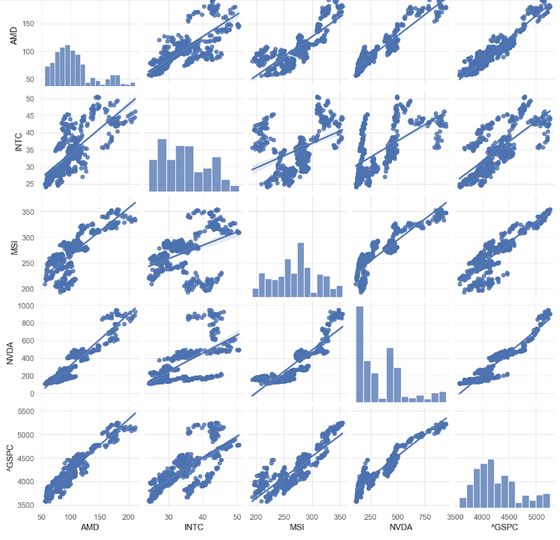
- Plotting the stock correlation matrix
# Correlation Matrix
corr = df.corr()
mask = np.zeros_like(corr)
mask[np.triu_indices_from(mask)] = True
sns.heatmap(corr, annot=True, mask = mask)
plt.show()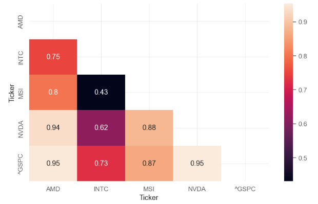
Key Technical Indicators
- Adding Technical Indicators (TI) to gain more insights into the supply and demand of our securities.
- NVDA candlesticks with key TI
start='2023-01-01'
# Downloading Stocks
nvda = yf.download('NVDA', start = start)

# Adding Moving Averages
nvda['EMA9'] = nvda['Adj Close'].ewm(span = 9, adjust = False).mean() # Exponential 9-Period Moving Average
nvda['SMA20'] = nvda['Adj Close'].rolling(window=20).mean() # Simple 20-Period Moving Average
nvda['SMA50'] = nvda['Adj Close'].rolling(window=50).mean() # Simple 50-Period Moving Average
nvda['SMA100'] = nvda['Adj Close'].rolling(window=100).mean() # Simple 100-Period Moving Average
nvda['SMA200'] = nvda['Adj Close'].rolling(window=200).mean() # Simple 200-Period Moving Average

# Adding RSI for 14-periods
delta = nvda['Adj Close'].diff() # Calculating delta
gain = delta.where(delta > 0,0) # Obtaining gain values
loss = -delta.where(delta < 0,0) # Obtaining loss values
avg_gain = gain.rolling(window=14).mean() # Measuring the 14-period average gain value
avg_loss = loss.rolling(window=14).mean() # Measuring the 14-period average loss value
rs = avg_gain/avg_loss # Calculating the RS
nvda['RSI'] = 100 - (100 / (1 + rs)) # Creating an RSI column to the Data Frame

# Adding Bollinger Bands 20-periods
nvda['BB_UPPER'] = nvda['SMA20'] + 2*nvda['Adj Close'].rolling(window=20).std() # Upper Band
nvda['BB_LOWER'] = nvda['SMA20'] - 2*nvda['Adj Close'].rolling(window=20).std() # Lower Band

# Adding ATR 14-periods
nvda['TR'] = pd.DataFrame(np.maximum(np.maximum(nvda['High'] - nvda['Low'], abs(nvda['High'] - nvda['Adj Close'].shift())), abs(nvda['Low'] - nvda['Adj Close'].shift())), index = nvda.index)
nvda['ATR'] = nvda['TR'].rolling(window = 14).mean() # Creating an ART column to the Data Frame

# Plotting Candlestick charts with indicators
fig = make_subplots(rows=4, cols=1, shared_xaxes=True, vertical_spacing=0.05,row_heights=[0.6, 0.10, 0.10, 0.20])

# Candlestick
fig.add_trace(go.Candlestick(x=nvda.index,
                             open=nvda['Open'],
                             high=nvda['High'],
                             low=nvda['Low'],
                             close=nvda['Adj Close'],
                             name='NVDA'),
              row=1, col=1)

# Moving Averages
fig.add_trace(go.Scatter(x=nvda.index,
                         y=nvda['EMA9'],
                         mode='lines',
                         line=dict(color='#90EE90'),
                         name='EMA9'),
              row=1, col=1)

fig.add_trace(go.Scatter(x=nvda.index,
                         y=nvda['SMA20'],
                         mode='lines',
                         line=dict(color='yellow'),
                         name='SMA20'),
              row=1, col=1)

fig.add_trace(go.Scatter(x=nvda.index,
                         y=nvda['SMA50'],
                         mode='lines',
                         line=dict(color='orange'),
                         name='SMA50'),
              row=1, col=1)

fig.add_trace(go.Scatter(x=nvda.index,
                         y=nvda['SMA100'],
                         mode='lines',
                         line=dict(color='purple'),
                         name='SMA100'),
              row=1, col=1)

fig.add_trace(go.Scatter(x=nvda.index,
                         y=nvda['SMA200'],
                         mode='lines',
                         line=dict(color='red'),
                         name='SMA200'),
              row=1, col=1)

# Bollinger Bands
fig.add_trace(go.Scatter(x=nvda.index,
                         y=nvda['BB_UPPER'],
                         mode='lines',
                         line=dict(color='#00BFFF'),
                         name='Upper Band'),
              row=1, col=1)

fig.add_trace(go.Scatter(x=nvda.index,
                         y=nvda['BB_LOWER'],
                         mode='lines',
                         line=dict(color='#00BFFF'),
                         name='Lower Band'),
              row=1, col=1)

fig.add_annotation(text='NVDA',
                    font=dict(color='white', size=40),
                    xref='paper', yref='paper',
                    x=0.5, y=0.65,
                    showarrow=False,
                    opacity=0.2)


# Relative Strengh Index (RSI)
fig.add_trace(go.Scatter(x=nvda.index,
                         y=nvda['RSI'],
                         mode='lines',
                         line=dict(color='#CBC3E3'),
                         name='RSI'),
              row=2, col=1)

# Adding marking lines at 70 and 30 levels
fig.add_shape(type="line",
              x0=nvda.index[0], y0=70, x1=nvda.index[-1], y1=70,
              line=dict(color="red", width=2, dash="dot"),
              row=2, col=1)
fig.add_shape(type="line",
              x0=nvda.index[0], y0=30, x1=nvda.index[-1], y1=30,
              line=dict(color="#90EE90", width=2, dash="dot"),
              row=2, col=1)

# Average True Range (ATR)
fig.add_trace(go.Scatter(x=nvda.index,
                         y=nvda['ATR'],
                         mode='lines',
                         line=dict(color='#00BFFF'),
                         name='ATR'),
              row=3, col=1)


# Volume
fig.add_trace(go.Bar(x=nvda.index,
                     y=nvda['Volume'],
                     name='Volume',
                     marker=dict(color='orange', opacity=1.0)),
              row=4, col=1)


# Layout
fig.update_layout(title='NVDA Candlestick Chart',
                  yaxis=dict(title='Price (USD)'),
                  height=1000,
                 template = 'plotly_dark')

# Axes and subplots
fig.update_xaxes(rangeslider_visible=False, row=1, col=1)
fig.update_xaxes(rangeslider_visible=False, row=4, col=1)
fig.update_yaxes(title_text='Price (USD)', row=1, col=1)
fig.update_yaxes(title_text='RSI', row=2, col=1)
fig.update_yaxes(title_text='ATR', row=3, col=1)
fig.update_yaxes(title_text='Volume', row=4, col=1)

fig.show()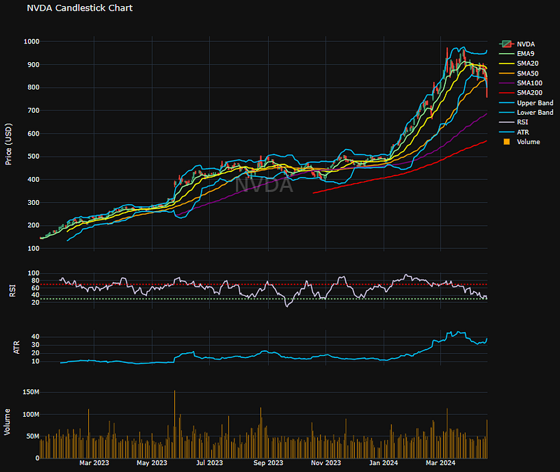
- AMD candlesticks with key TI
start='2023-01-01'
# Downloading Stocks
nvda = yf.download('AMD', start = start)
# Adding Moving Averages
nvda['EMA9'] = nvda['Adj Close'].ewm(span = 9, adjust = False).mean() # Exponential 9-Period Moving Average
nvda['SMA20'] = nvda['Adj Close'].rolling(window=20).mean() # Simple 20-Period Moving Average
nvda['SMA50'] = nvda['Adj Close'].rolling(window=50).mean() # Simple 50-Period Moving Average
nvda['SMA100'] = nvda['Adj Close'].rolling(window=100).mean() # Simple 100-Period Moving Average
nvda['SMA200'] = nvda['Adj Close'].rolling(window=200).mean() # Simple 200-Period Moving Average

# Adding RSI for 14-periods
delta = nvda['Adj Close'].diff() # Calculating delta
gain = delta.where(delta > 0,0) # Obtaining gain values
loss = -delta.where(delta < 0,0) # Obtaining loss values
avg_gain = gain.rolling(window=14).mean() # Measuring the 14-period average gain value
avg_loss = loss.rolling(window=14).mean() # Measuring the 14-period average loss value
rs = avg_gain/avg_loss # Calculating the RS
nvda['RSI'] = 100 - (100 / (1 + rs)) # Creating an RSI column to the Data Frame

# Adding Bollinger Bands 20-periods
nvda['BB_UPPER'] = nvda['SMA20'] + 2*nvda['Adj Close'].rolling(window=20).std() # Upper Band
nvda['BB_LOWER'] = nvda['SMA20'] - 2*nvda['Adj Close'].rolling(window=20).std() # Lower Band

# Adding ATR 14-periods
nvda['TR'] = pd.DataFrame(np.maximum(np.maximum(nvda['High'] - nvda['Low'], abs(nvda['High'] - nvda['Adj Close'].shift())), abs(nvda['Low'] - nvda['Adj Close'].shift())), index = nvda.index)
nvda['ATR'] = nvda['TR'].rolling(window = 14).mean() # Creating an ART column to the Data Frame

# Plotting Candlestick charts with indicators
fig = make_subplots(rows=4, cols=1, shared_xaxes=True, vertical_spacing=0.05,row_heights=[0.6, 0.10, 0.10, 0.20])

# Candlestick
fig.add_trace(go.Candlestick(x=nvda.index,
                             open=nvda['Open'],
                             high=nvda['High'],
                             low=nvda['Low'],
                             close=nvda['Adj Close'],
                             name='AMD'),
              row=1, col=1)

# Moving Averages
fig.add_trace(go.Scatter(x=nvda.index,
                         y=nvda['EMA9'],
                         mode='lines',
                         line=dict(color='#90EE90'),
                         name='EMA9'),
              row=1, col=1)

fig.add_trace(go.Scatter(x=nvda.index,
                         y=nvda['SMA20'],
                         mode='lines',
                         line=dict(color='yellow'),
                         name='SMA20'),
              row=1, col=1)

fig.add_trace(go.Scatter(x=nvda.index,
                         y=nvda['SMA50'],
                         mode='lines',
                         line=dict(color='orange'),
                         name='SMA50'),
              row=1, col=1)

fig.add_trace(go.Scatter(x=nvda.index,
                         y=nvda['SMA100'],
                         mode='lines',
                         line=dict(color='purple'),
                         name='SMA100'),
              row=1, col=1)

fig.add_trace(go.Scatter(x=nvda.index,
                         y=nvda['SMA200'],
                         mode='lines',
                         line=dict(color='red'),
                         name='SMA200'),
              row=1, col=1)

# Bollinger Bands
fig.add_trace(go.Scatter(x=nvda.index,
                         y=nvda['BB_UPPER'],
                         mode='lines',
                         line=dict(color='#00BFFF'),
                         name='Upper Band'),
              row=1, col=1)

fig.add_trace(go.Scatter(x=nvda.index,
                         y=nvda['BB_LOWER'],
                         mode='lines',
                         line=dict(color='#00BFFF'),
                         name='Lower Band'),
              row=1, col=1)

fig.add_annotation(text='AMD',
                    font=dict(color='white', size=40),
                    xref='paper', yref='paper',
                    x=0.5, y=0.65,
                    showarrow=False,
                    opacity=0.2)


# Relative Strengh Index (RSI)
fig.add_trace(go.Scatter(x=nvda.index,
                         y=nvda['RSI'],
                         mode='lines',
                         line=dict(color='#CBC3E3'),
                         name='RSI'),
              row=2, col=1)

# Adding marking lines at 70 and 30 levels
fig.add_shape(type="line",
              x0=nvda.index[0], y0=70, x1=nvda.index[-1], y1=70,
              line=dict(color="red", width=2, dash="dot"),
              row=2, col=1)
fig.add_shape(type="line",
              x0=nvda.index[0], y0=30, x1=nvda.index[-1], y1=30,
              line=dict(color="#90EE90", width=2, dash="dot"),
              row=2, col=1)

# Average True Range (ATR)
fig.add_trace(go.Scatter(x=nvda.index,
                         y=nvda['ATR'],
                         mode='lines',
                         line=dict(color='#00BFFF'),
                         name='ATR'),
              row=3, col=1)


# Volume
fig.add_trace(go.Bar(x=nvda.index,
                     y=nvda['Volume'],
                     name='Volume',
                     marker=dict(color='orange', opacity=1.0)),
              row=4, col=1)


# Layout
fig.update_layout(title='AMD Candlestick Chart',
                  yaxis=dict(title='Price (USD)'),
                  height=1000,
                 template = 'plotly_dark')

# Axes and subplots
fig.update_xaxes(rangeslider_visible=False, row=1, col=1)
fig.update_xaxes(rangeslider_visible=False, row=4, col=1)
fig.update_yaxes(title_text='Price (USD)', row=1, col=1)
fig.update_yaxes(title_text='RSI', row=2, col=1)
fig.update_yaxes(title_text='ATR', row=3, col=1)
fig.update_yaxes(title_text='Volume', row=4, col=1)

fig.show()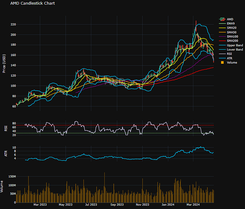
- MSI candlesticks with key TI
start='2023-01-01'
# Downloading Stocks
nvda = yf.download('MSI', start = start)
# Adding Moving Averages
nvda['EMA9'] = nvda['Adj Close'].ewm(span = 9, adjust = False).mean() # Exponential 9-Period Moving Average
nvda['SMA20'] = nvda['Adj Close'].rolling(window=20).mean() # Simple 20-Period Moving Average
nvda['SMA50'] = nvda['Adj Close'].rolling(window=50).mean() # Simple 50-Period Moving Average
nvda['SMA100'] = nvda['Adj Close'].rolling(window=100).mean() # Simple 100-Period Moving Average
nvda['SMA200'] = nvda['Adj Close'].rolling(window=200).mean() # Simple 200-Period Moving Average

# Adding RSI for 14-periods
delta = nvda['Adj Close'].diff() # Calculating delta
gain = delta.where(delta > 0,0) # Obtaining gain values
loss = -delta.where(delta < 0,0) # Obtaining loss values
avg_gain = gain.rolling(window=14).mean() # Measuring the 14-period average gain value
avg_loss = loss.rolling(window=14).mean() # Measuring the 14-period average loss value
rs = avg_gain/avg_loss # Calculating the RS
nvda['RSI'] = 100 - (100 / (1 + rs)) # Creating an RSI column to the Data Frame

# Adding Bollinger Bands 20-periods
nvda['BB_UPPER'] = nvda['SMA20'] + 2*nvda['Adj Close'].rolling(window=20).std() # Upper Band
nvda['BB_LOWER'] = nvda['SMA20'] - 2*nvda['Adj Close'].rolling(window=20).std() # Lower Band

# Adding ATR 14-periods
nvda['TR'] = pd.DataFrame(np.maximum(np.maximum(nvda['High'] - nvda['Low'], abs(nvda['High'] - nvda['Adj Close'].shift())), abs(nvda['Low'] - nvda['Adj Close'].shift())), index = nvda.index)
nvda['ATR'] = nvda['TR'].rolling(window = 14).mean() # Creating an ART column to the Data Frame

# Plotting Candlestick charts with indicators
fig = make_subplots(rows=4, cols=1, shared_xaxes=True, vertical_spacing=0.05,row_heights=[0.6, 0.10, 0.10, 0.20])

# Candlestick
fig.add_trace(go.Candlestick(x=nvda.index,
                             open=nvda['Open'],
                             high=nvda['High'],
                             low=nvda['Low'],
                             close=nvda['Adj Close'],
                             name='MSI'),
              row=1, col=1)

# Moving Averages
fig.add_trace(go.Scatter(x=nvda.index,
                         y=nvda['EMA9'],
                         mode='lines',
                         line=dict(color='#90EE90'),
                         name='EMA9'),
              row=1, col=1)

fig.add_trace(go.Scatter(x=nvda.index,
                         y=nvda['SMA20'],
                         mode='lines',
                         line=dict(color='yellow'),
                         name='SMA20'),
              row=1, col=1)

fig.add_trace(go.Scatter(x=nvda.index,
                         y=nvda['SMA50'],
                         mode='lines',
                         line=dict(color='orange'),
                         name='SMA50'),
              row=1, col=1)

fig.add_trace(go.Scatter(x=nvda.index,
                         y=nvda['SMA100'],
                         mode='lines',
                         line=dict(color='purple'),
                         name='SMA100'),
              row=1, col=1)

fig.add_trace(go.Scatter(x=nvda.index,
                         y=nvda['SMA200'],
                         mode='lines',
                         line=dict(color='red'),
                         name='SMA200'),
              row=1, col=1)

# Bollinger Bands
fig.add_trace(go.Scatter(x=nvda.index,
                         y=nvda['BB_UPPER'],
                         mode='lines',
                         line=dict(color='#00BFFF'),
                         name='Upper Band'),
              row=1, col=1)

fig.add_trace(go.Scatter(x=nvda.index,
                         y=nvda['BB_LOWER'],
                         mode='lines',
                         line=dict(color='#00BFFF'),
                         name='Lower Band'),
              row=1, col=1)

fig.add_annotation(text='MSI',
                    font=dict(color='white', size=40),
                    xref='paper', yref='paper',
                    x=0.5, y=0.65,
                    showarrow=False,
                    opacity=0.2)


# Relative Strengh Index (RSI)
fig.add_trace(go.Scatter(x=nvda.index,
                         y=nvda['RSI'],
                         mode='lines',
                         line=dict(color='#CBC3E3'),
                         name='RSI'),
              row=2, col=1)

# Adding marking lines at 70 and 30 levels
fig.add_shape(type="line",
              x0=nvda.index[0], y0=70, x1=nvda.index[-1], y1=70,
              line=dict(color="red", width=2, dash="dot"),
              row=2, col=1)
fig.add_shape(type="line",
              x0=nvda.index[0], y0=30, x1=nvda.index[-1], y1=30,
              line=dict(color="#90EE90", width=2, dash="dot"),
              row=2, col=1)

# Average True Range (ATR)
fig.add_trace(go.Scatter(x=nvda.index,
                         y=nvda['ATR'],
                         mode='lines',
                         line=dict(color='#00BFFF'),
                         name='ATR'),
              row=3, col=1)


# Volume
fig.add_trace(go.Bar(x=nvda.index,
                     y=nvda['Volume'],
                     name='Volume',
                     marker=dict(color='orange', opacity=1.0)),
              row=4, col=1)


# Layout
fig.update_layout(title='MSI Candlestick Chart',
                  yaxis=dict(title='Price (USD)'),
                  height=1000,
                 template = 'plotly_dark')

# Axes and subplots
fig.update_xaxes(rangeslider_visible=False, row=1, col=1)
fig.update_xaxes(rangeslider_visible=False, row=4, col=1)
fig.update_yaxes(title_text='Price (USD)', row=1, col=1)
fig.update_yaxes(title_text='RSI', row=2, col=1)
fig.update_yaxes(title_text='ATR', row=3, col=1)
fig.update_yaxes(title_text='Volume', row=4, col=1)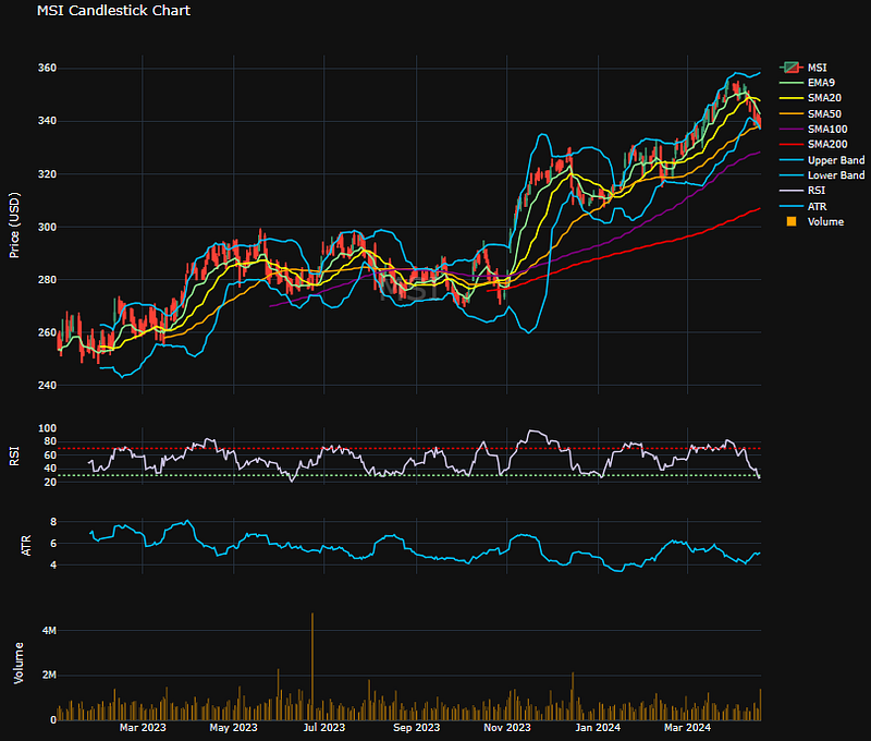
- INTC candlesticks with key TI
start='2023-01-01'
# Downloading Stocks
nvda = yf.download('INTC', start = start)
# Adding Moving Averages
nvda['EMA9'] = nvda['Adj Close'].ewm(span = 9, adjust = False).mean() # Exponential 9-Period Moving Average
nvda['SMA20'] = nvda['Adj Close'].rolling(window=20).mean() # Simple 20-Period Moving Average
nvda['SMA50'] = nvda['Adj Close'].rolling(window=50).mean() # Simple 50-Period Moving Average
nvda['SMA100'] = nvda['Adj Close'].rolling(window=100).mean() # Simple 100-Period Moving Average
nvda['SMA200'] = nvda['Adj Close'].rolling(window=200).mean() # Simple 200-Period Moving Average

# Adding RSI for 14-periods
delta = nvda['Adj Close'].diff() # Calculating delta
gain = delta.where(delta > 0,0) # Obtaining gain values
loss = -delta.where(delta < 0,0) # Obtaining loss values
avg_gain = gain.rolling(window=14).mean() # Measuring the 14-period average gain value
avg_loss = loss.rolling(window=14).mean() # Measuring the 14-period average loss value
rs = avg_gain/avg_loss # Calculating the RS
nvda['RSI'] = 100 - (100 / (1 + rs)) # Creating an RSI column to the Data Frame

# Adding Bollinger Bands 20-periods
nvda['BB_UPPER'] = nvda['SMA20'] + 2*nvda['Adj Close'].rolling(window=20).std() # Upper Band
nvda['BB_LOWER'] = nvda['SMA20'] - 2*nvda['Adj Close'].rolling(window=20).std() # Lower Band

# Adding ATR 14-periods
nvda['TR'] = pd.DataFrame(np.maximum(np.maximum(nvda['High'] - nvda['Low'], abs(nvda['High'] - nvda['Adj Close'].shift())), abs(nvda['Low'] - nvda['Adj Close'].shift())), index = nvda.index)
nvda['ATR'] = nvda['TR'].rolling(window = 14).mean() # Creating an ART column to the Data Frame

# Plotting Candlestick charts with indicators
fig = make_subplots(rows=4, cols=1, shared_xaxes=True, vertical_spacing=0.05,row_heights=[0.6, 0.10, 0.10, 0.20])

# Candlestick
fig.add_trace(go.Candlestick(x=nvda.index,
                             open=nvda['Open'],
                             high=nvda['High'],
                             low=nvda['Low'],
                             close=nvda['Adj Close'],
                             name='INTC'),
              row=1, col=1)

# Moving Averages
fig.add_trace(go.Scatter(x=nvda.index,
                         y=nvda['EMA9'],
                         mode='lines',
                         line=dict(color='#90EE90'),
                         name='EMA9'),
              row=1, col=1)

fig.add_trace(go.Scatter(x=nvda.index,
                         y=nvda['SMA20'],
                         mode='lines',
                         line=dict(color='yellow'),
                         name='SMA20'),
              row=1, col=1)

fig.add_trace(go.Scatter(x=nvda.index,
                         y=nvda['SMA50'],
                         mode='lines',
                         line=dict(color='orange'),
                         name='SMA50'),
              row=1, col=1)

fig.add_trace(go.Scatter(x=nvda.index,
                         y=nvda['SMA100'],
                         mode='lines',
                         line=dict(color='purple'),
                         name='SMA100'),
              row=1, col=1)

fig.add_trace(go.Scatter(x=nvda.index,
                         y=nvda['SMA200'],
                         mode='lines',
                         line=dict(color='red'),
                         name='SMA200'),
              row=1, col=1)

# Bollinger Bands
fig.add_trace(go.Scatter(x=nvda.index,
                         y=nvda['BB_UPPER'],
                         mode='lines',
                         line=dict(color='#00BFFF'),
                         name='Upper Band'),
              row=1, col=1)

fig.add_trace(go.Scatter(x=nvda.index,
                         y=nvda['BB_LOWER'],
                         mode='lines',
                         line=dict(color='#00BFFF'),
                         name='Lower Band'),
              row=1, col=1)

fig.add_annotation(text='INTC',
                    font=dict(color='white', size=40),
                    xref='paper', yref='paper',
                    x=0.5, y=0.65,
                    showarrow=False,
                    opacity=0.2)


# Relative Strengh Index (RSI)
fig.add_trace(go.Scatter(x=nvda.index,
                         y=nvda['RSI'],
                         mode='lines',
                         line=dict(color='#CBC3E3'),
                         name='RSI'),
              row=2, col=1)

# Adding marking lines at 70 and 30 levels
fig.add_shape(type="line",
              x0=nvda.index[0], y0=70, x1=nvda.index[-1], y1=70,
              line=dict(color="red", width=2, dash="dot"),
              row=2, col=1)
fig.add_shape(type="line",
              x0=nvda.index[0], y0=30, x1=nvda.index[-1], y1=30,
              line=dict(color="#90EE90", width=2, dash="dot"),
              row=2, col=1)

# Average True Range (ATR)
fig.add_trace(go.Scatter(x=nvda.index,
                         y=nvda['ATR'],
                         mode='lines',
                         line=dict(color='#00BFFF'),
                         name='ATR'),
              row=3, col=1)


# Volume
fig.add_trace(go.Bar(x=nvda.index,
                     y=nvda['Volume'],
                     name='Volume',
                     marker=dict(color='orange', opacity=1.0)),
              row=4, col=1)


# Layout
fig.update_layout(title='INTC Candlestick Chart',
                  yaxis=dict(title='Price (USD)'),
                  height=1000,
                 template = 'plotly_dark')

# Axes and subplots
fig.update_xaxes(rangeslider_visible=False, row=1, col=1)
fig.update_xaxes(rangeslider_visible=False, row=4, col=1)
fig.update_yaxes(title_text='Price (USD)', row=1, col=1)
fig.update_yaxes(title_text='RSI', row=2, col=1)
fig.update_yaxes(title_text='ATR', row=3, col=1)
fig.update_yaxes(title_text='Volume', row=4, col=1)
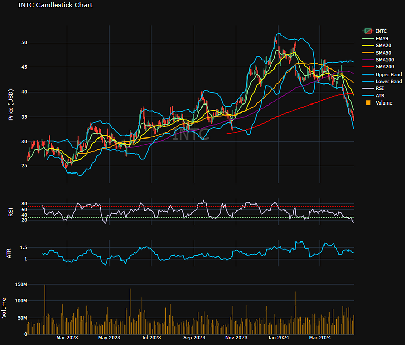
Backtesting INTC Trading Strategies
- The above INTC candlesticks with key TI suggest that we need to outperform the passive buy-and-hold strategy of this stock. In doing so, we will implement and backtest the following TI-based trading strategies
# Importing necessary libraries
import pandas as pd
import numpy as np
import matplotlib.pyplot as plt
import yfinance as yf
import pyfolio as pf
import datetime as dt

import os
import warnings

# print all outputs
from IPython.core.interactiveshell import InteractiveShell
InteractiveShell.ast_node_interactivity = "all"

# downloading historical necessary data for backtesting and analysis
_start = dt.date(2022,1,2)
_end = dt.date(2024,4,20)
ticker = 'INTC'
df = yf.download(ticker, start = _start, end = _end)
#df.tail()

# calculating buy and hold strategy returns
df['bnh_returns'] = np.log(df['Adj Close']/df['Adj Close'].shift(1))

# creating bollinger band indicators
df['ma20'] = df['Adj Close'].rolling(window=20).mean()
df['std'] = df['Adj Close'].rolling(window=20).std()
df['upper_band'] = df['ma20'] + (2 * df['std'])
df['lower_band'] = df['ma20'] - (2 * df['std'])
df.drop(['Open','High','Low'],axis=1,inplace=True,errors='ignore')
#df.tail(5)

# BUY condition
df['signal'] = np.where((df['Adj Close'] < df['lower_band']) &
                        (df['Adj Close'].shift(1) >=       df['lower_band']),1,0)

# SELL condition
df['signal'] = np.where( (df['Adj Close'] > df['upper_band']) &
                          (df['Adj Close'].shift(1) <= df['upper_band']),-1,df['signal'])
# creating long and short positions
df['position'] = df['signal'].replace(to_replace=0, method='ffill')

# shifting by 1, to account of close price return calculations
df['position'] = df['position'].shift(1)

# calculating stretegy returns
df['strategy_returns'] = df['bnh_returns'] * (df['position'])

#df.tail(5)

# comparing buy & hold strategy / bollinger bands strategy returns
print("Buy and hold returns:",df['bnh_returns'].cumsum()[-1])
print("Strategy returns:",df['strategy_returns'].cumsum()[-1])

# plotting strategy historical performance over time
df[['bnh_returns','strategy_returns']] = df[['bnh_returns','strategy_returns']].cumsum()
df[['bnh_returns','strategy_returns']].plot(grid=True, figsize=(12, 8))

Buy and hold returns: -0.3770989996574775
Strategy returns: 1.3603005119382139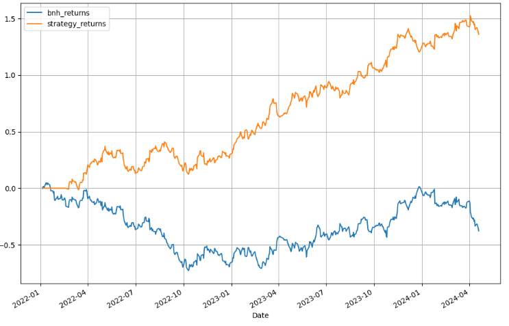
- Printing pyfolio strategy QC diagnostics
import pyfolio as pf
pf.create_simple_tear_sheet(df['strategy_returns'].diff())

Start date 2022-01-03
End date 2024-04-19
Total months 27
Backtest
Annual return 68.595%
Cumulative returns 230.676%
Annual volatility 38.018%
Sharpe ratio 1.57
Calmar ratio 2.68
Stability 0.92
Max drawdown -25.626%
Omega ratio 1.31
Sortino ratio 2.56
Skew NaN
Kurtosis NaN
Tail ratio 1.26
Daily value at risk -4.553%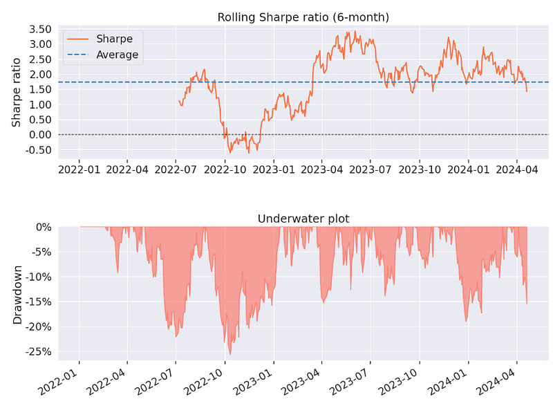
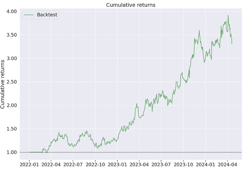
- Plotting INTC backtesting trading signals, BB, MA20 and Close price
df.tail()
           Close    Adj Close    Volume bnh_returns ma20  std  upper_band lower_band signal position strategy_returns
Date
2024-04-15 36.310001 36.310001 50751600 -0.317231 40.7040 2.792515 46.289030 35.118970 0 1.0 1.420168
2024-04-16 36.259998 36.259998 30607500 -0.318610 40.3815 2.918270 46.218039 34.544961 0 1.0 1.418790
2024-04-17 35.680000 35.680000 41173300 -0.334734 40.0630 3.070239 46.203479 33.922522 0 1.0 1.402665
2024-04-18 35.040001 35.040001 42334400 -0.352834 39.7050 3.221649 46.148299 33.261701 0 1.0 1.384565
2024-04-19 34.200001 34.200001 58968800 -0.377099 39.2940 3.377611 46.049222 32.538778 0 1.0 1.360301

buy_price = []
sell_price = []
prices=df['Close']
for i in range(len(prices)):
    if df['signal'][i] > 0.0:
        buy_price.append(prices[i])
        sell_price.append(np.nan)
    if df['signal'][i] < 0.0:
        sell_price.append(prices[i])
        buy_price.append(np.nan)
    if df["signal"][i] == 0.0:
        sell_price.append(np.nan)
        buy_price.append(np.nan)

plt.figure(figsize=(12,7))
plt.plot(df["Close"], color="black", label="Price")
plt.plot(df.index, buy_price, marker = '^', markersize = 8, color = 'green', linewidth = 0, label = 'BUY SIGNAL')
plt.plot(df.index, sell_price, marker = 'v', markersize = 8, color = 'r', linewidth = 0, label = 'SELL SIGNAL')
plt.plot(df["upper_band"], color="blue", label="Upper BB")
plt.plot(df["lower_band"], color="green", label="Lower BB")
plt.plot(df["ma20"], color="orange", label="MA20")
plt.legend()
plt.grid()
plt.title("Backtesting INTC TI Trading Strategy",fontsize=16)
plt.xlabel("Date",fontsize=16)
plt.ylabel("Close Price USD",fontsize=16)
plt.show()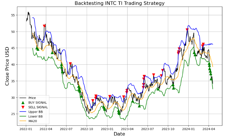
- Comparing these results to the ^GSPC cumulative returns
# downloading historical necessary data for backtesting and analysis
_start = dt.date(2022,1,2)
_end = dt.date(2024,4,20)
ticker = '^GSPC'
dfg = yf.download(ticker, start = _start, end = _end)
# calculating buy and hold strategy returns
dfg['bnh_returns'] = np.log(dfg['Adj Close']/dfg['Adj Close'].shift(1))
#dfg.tail(3)
print("^GSPC Buy and Hold returns:",dfg['bnh_returns'].cumsum()[-1])

dfg['daily_return'] = dfg['Close'].pct_change()
# calculate cumluative return
dfg['cum_return'] = np.exp(np.log1p(dfg['daily_return']).cumsum())
print (dfg['cum_return'])
dfg['cum_return'].plot()

^GSPC Buy and Hold returns: 0.03496333020354546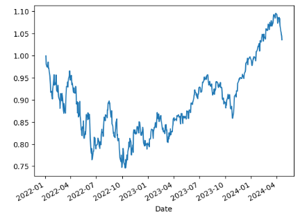
SciPy Portfolio Optimization
- Let’s consider several popular stochastic simulation techniques of creating an optimized portfolio of our 4 tech assets, for which our investment strategy has the maximum return and minimum risk or max(ROI/Risk) as compared to the S&P 500 benchmark.
- For example, the Markowitz Mean-Variance Optimization Model is a widely-used framework for constructing portfolios with the best risk-return relationship.
- Firstly, we estimate expected returns using daily prices as input.
- Secondly, we invoke the covariance matrix as the most commonly used risk model.
- Read more about the implemented scipy optimization algorithm and the related PO guide for data scientists.
#Importing Libraries
import numpy as np
import pandas as pd
import yfinance as yf
import matplotlib.pyplot as plt
from scipy.optimize import minimize
from scipy.stats import norm
from scipy.stats import skew, kurtosis
from scipy.stats.mstats import gmean
# Select Optimization Criteria 'sharpe', 'cvar', 'sortino' or 'variance'
optimization_criterion = 'cvar'

#Read input Adj Close prices
symbols = ['NVDA', 'AMD', 'MSI', 'INTC']
start_date = '2022-01-01'
end_date = '2024-04-20'

data = yf.download(symbols, start=start_date, end=end_date)['Adj Close']
data.tail()
Ticker AMD INTC MSI NVDA
Date
2024-04-15 160.320007 36.310001 338.579987 860.010010
2024-04-16 163.460007 36.259998 340.109985 874.150024
2024-04-17 154.020004 35.680000 340.510010 840.349976
2024-04-18 155.080002 35.040001 339.459991 846.710022
2024-04-19 146.639999 34.200001 339.649994 762.000000

#Calculate daily returns
returns = data.pct_change().dropna()- Defining the optimization objective functions , constraints and bounds
def objective_sharpe(weights):
    return -np.dot(weights, returns.mean()) / np.sqrt(np.dot(weights.T, np.dot(returns.cov() * 252, weights)))
def objective_cvar(weights):
    portfolio_returns = np.dot(returns, weights)
    portfolio_mean = portfolio_returns.mean()
    portfolio_std = portfolio_returns.std()
    conf_level = 0.05  # Confidence level
    cvar = portfolio_mean - portfolio_std * norm.ppf(conf_level)
    return cvar
def objective_sortino(weights):
    portfolio_returns = np.dot(returns, weights)
    downside_returns = portfolio_returns[portfolio_returns < 0]
    downside_std = downside_returns.std()
    sortino_ratio = portfolio_returns.mean() / downside_std
    return -sortino_ratio
def objective_variance(weights):
    return np.dot(weights.T, np.dot(returns.cov() * 252, weights))

cons = ({'type': 'eq', 'fun': lambda x: np.sum(x) - 1})
bounds = tuple((0, 1) for x in range(len(symbols)))- Running the PO algorithm with optimal weights
# Optimization
init_guess = np.array(len(symbols) * [1. / len(symbols),])
if optimization_criterion == 'sharpe':
    opt_results = minimize(objective_sharpe, init_guess, method='SLSQP', bounds=bounds, constraints=cons)
elif optimization_criterion == 'cvar':
    opt_results = minimize(objective_cvar, init_guess, method='SLSQP', bounds=bounds, constraints=cons)
elif optimization_criterion == 'sortino':
    opt_results = minimize(objective_sortino, init_guess, method='SLSQP', bounds=bounds, constraints=cons)
elif optimization_criterion == 'variance':
    opt_results = minimize(objective_variance, init_guess, method='SLSQP', bounds=bounds, constraints=cons)

# Optimal weights
optimal_weights = opt_results.x


# Optimize all criteria
opt_results_cvar = minimize(objective_cvar, init_guess, method='SLSQP', bounds=bounds, constraints=cons)
opt_results_sortino = minimize(objective_sortino, init_guess, method='SLSQP', bounds=bounds, constraints=cons)
opt_results_variance = minimize(objective_variance, init_guess, method='SLSQP', bounds=bounds, constraints=cons)
opt_results_sharpe = minimize(objective_sharpe, init_guess, method='SLSQP', bounds=bounds, constraints=cons)

# Optimal weights for each criterion
optimal_weights_cvar = opt_results_cvar.x
optimal_weights_sortino = opt_results_sortino.x
optimal_weights_variance = opt_results_variance.x
optimal_weights_sharpe = opt_results_sharpe.x- Plotting the efficient frontier
port_returns = []
port_volatility = []
sharpe_ratio = []
all_weights = []  # almacena los pesos de todas las carteras simuladas

num_assets = len(symbols)
num_portfolios = 50000

np.random.seed(101)

for single_portfolio in range(num_portfolios):
    weights = np.random.random(num_assets)
    weights /= np.sum(weights)
    returns_portfolio = np.dot(weights, returns.mean()) * 252
    volatility = np.sqrt(np.dot(weights.T, np.dot(returns.cov() * 252, weights)))
    sr = returns_portfolio / volatility
    sharpe_ratio.append(sr)
    port_returns.append(returns_portfolio)
    port_volatility.append(volatility)
    all_weights.append(weights)  # registra los pesos para esta cartera

plt.figure(figsize=(12, 8))
plt.scatter(port_volatility, port_returns, c=sharpe_ratio, cmap='viridis')
plt.colorbar(label='Sharpe Ratio')
plt.xlabel('Volatility',fontsize=14)
plt.ylabel('Return',fontsize=14)
plt.grid()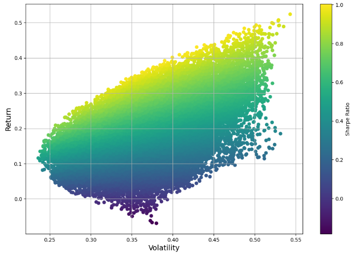
- Plotting the optimal portfolio for each criterion in the above domain
plt.figure(figsize=(12, 8))
plt.scatter(port_volatility, port_returns, c=sharpe_ratio, cmap='viridis')

opt_returns_cvar = np.dot(optimal_weights_cvar, returns.mean()) * 252
opt_volatility_cvar = np.sqrt(np.dot(optimal_weights_cvar.T, np.dot(returns.cov() * 252, optimal_weights_cvar)))
opt_portfolio_cvar = plt.scatter(opt_volatility_cvar, opt_returns_cvar, color='hotpink', s=250, label='CVaR')

opt_returns_sortino = np.dot(optimal_weights_sortino, returns.mean()) * 252
opt_volatility_sortino = np.sqrt(np.dot(optimal_weights_sortino.T, np.dot(returns.cov() * 252, optimal_weights_sortino)))
opt_portfolio_sortino = plt.scatter(opt_volatility_sortino, opt_returns_sortino, color='g', s=50, label='Sortino')

opt_returns_variance = np.dot(optimal_weights_variance, returns.mean()) * 252
opt_volatility_variance = np.sqrt(np.dot(optimal_weights_variance.T, np.dot(returns.cov() * 252, optimal_weights_variance)))
opt_portfolio_variance = plt.scatter(opt_volatility_variance, opt_returns_variance, color='b', s=50, label='Variance')

opt_returns_sharpe = np.dot(optimal_weights_sharpe, returns.mean()) * 252
opt_volatility_sharpe = np.sqrt(np.dot(optimal_weights_sharpe.T, np.dot(returns.cov() * 252, optimal_weights_sharpe)))
opt_portfolio_sharpe = plt.scatter(opt_volatility_sharpe, opt_returns_sharpe, color='r', s=50, label='Sharpe')


plt.legend(loc='upper left')
plt.colorbar(label='Sharpe Ratio')
plt.xlabel('Volatility',fontsize=14)
plt.ylabel('Return',fontsize=14)
plt.grid()
plt.show()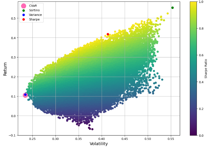
- Calculating and printing descriptive statistics of the optimized portfolios
# Function to calculate the maximum drawdown
def max_drawdown(return_series):
    comp_ret = (1 + return_series).cumprod()
    peak = comp_ret.expanding(min_periods=1).max()
    dd = (comp_ret/peak) - 1
    return dd.min()

# Function to calculate more detailed descriptive statistics
def detailed_portfolio_statistics(weights):
    portfolio_returns = returns.dot(weights)

    # General descriptive statistics
    mean_return_annualized = gmean(portfolio_returns + 1)**252 - 1
    std_dev_annualized = portfolio_returns.std() * np.sqrt(252)
    skewness = skew(portfolio_returns)
    kurt = kurtosis(portfolio_returns)
    max_dd = max_drawdown(portfolio_returns)
    count = len(portfolio_returns)

    # Optimization metrics
    risk_free_rate = 0.00
    sharpe_ratio = (mean_return_annualized - risk_free_rate) / std_dev_annualized
    conf_level = 0.05
    cvar = mean_return_annualized - std_dev_annualized * norm.ppf(conf_level)
    downside_returns = portfolio_returns[portfolio_returns < 0]
    downside_std_dev = downside_returns.std() * np.sqrt(252)
    sortino_ratio = mean_return_annualized / downside_std_dev
    variance = std_dev_annualized ** 2

    return mean_return_annualized, std_dev_annualized, skewness, kurt, max_dd, count, sharpe_ratio, cvar, sortino_ratio, variance

# Calculate statistics for each portfolioCalculate statistics for each portfolio
statistics_cvar = detailed_portfolio_statistics(optimal_weights_cvar)
statistics_sortino = detailed_portfolio_statistics(optimal_weights_sortino)
statistics_variance = detailed_portfolio_statistics(optimal_weights_variance)
statistics_sharpe = detailed_portfolio_statistics(optimal_weights_sharpe)

# Statistics names
statistics_names = ['Annualized return', 'Annualized volatility', 'Skewness', 'Kurtosis', 'Max Drawdown', 'Data content', 'Sharpe Ratio', 'CVaR', 'Sortino Ratio', 'Variance']

# Dictionary that associates the names of optimization methods with optimal weights and statistics
portfolio_data = {
    'CVaR': {
        'weights': optimal_weights_cvar,
        'statistics': detailed_portfolio_statistics(optimal_weights_cvar)
    },
    'Sortino': {
        'weights': optimal_weights_sortino,
        'statistics': detailed_portfolio_statistics(optimal_weights_sortino)
    },
    'Variance': {
        'weights': optimal_weights_variance,
        'statistics': detailed_portfolio_statistics(optimal_weights_variance)
    },
    'Sharpe': {
        'weights': optimal_weights_sharpe,
        'statistics': detailed_portfolio_statistics(optimal_weights_sharpe)
    },
}

# Print the weights and statistics for each optimization method
for method, data in portfolio_data.items():
    print("\n")
    print("========================================================================================================")
    print("\n")
    print(f"Optimum portfolio weights for {method}:")
    print("\n")
    for symbol, weight in zip(symbols, data['weights']):
        if weight < 1e-4:  # considers any weight less than 0.01% as zero
            print(f"{symbol}: practically 0%")
        else:
            print(f"{symbol}: {weight*100:.2f}%")

    print("\n")
    print(f"Descriptive statistics of the optimal portfolio for {method}:")
    print("\n")
    for name, stat in zip(statistics_names, data['statistics']):
        print(f"{name}: {stat*100 if name != 'Data content' else stat:.2f}")

print("\n")
print("========================================================================================================")
========================================================================================================
Optimum portfolio weights for CVaR:
NVDA: practically 0%
AMD: 17.51%
MSI: 82.49%
INTC: practically 0%
Descriptive statistics of the optimal portfolio for CVaR:
Annualized return: 8.12
Annualized volatility: 23.45
Skewness: 24.53
Kurtosis: 197.09
Max Drawdown: -25.46
Data content: 576.00
Sharpe Ratio: 34.63
CVaR: 46.69
Sortino Ratio: 54.29
Variance: 5.50
========================================================================================================
Optimum portfolio weights for Sortino:
NVDA: practically 0%
AMD: practically 0%
MSI: 1.76%
INTC: 98.24%
Descriptive statistics of the optimal portfolio for Sortino:
Annualized return: 49.73
Annualized volatility: 55.35
Skewness: 81.96
Kurtosis: 462.31
Max Drawdown: -61.07
Data content: 576.00
Sharpe Ratio: 89.84
CVaR: 140.77
Sortino Ratio: 158.52
Variance: 30.64
========================================================================================================
Optimum portfolio weights for Variance:
NVDA: practically 0%
AMD: 16.32%
MSI: 83.68%
INTC: practically 0%
Descriptive statistics of the optimal portfolio for Variance:
Annualized return: 8.43
Annualized volatility: 23.45
Skewness: 24.82
Kurtosis: 203.47
Max Drawdown: -25.43
Data content: 576.00
Sharpe Ratio: 35.94
CVaR: 46.99
Sortino Ratio: 56.28
Variance: 5.50
========================================================================================================
Optimum portfolio weights for Sharpe:
NVDA: practically 0%
AMD: practically 0%
MSI: 34.47%
INTC: 65.53%
Descriptive statistics of the optimal portfolio for Sharpe:
Annualized return: 39.65
Annualized volatility: 41.33
Skewness: 61.72
Kurtosis: 313.14
Max Drawdown: -49.28
Data content: 576.00
Sharpe Ratio: 95.93
CVaR: 107.64
Sortino Ratio: 163.20
Variance: 17.08
========================================================================================================Modern Port Monte Carlo Simulations
- Let’s delve into the specifics of Markowitz Portfolio Optimization (MPO) by employing the Monte Carlo simulations combined with relevant matplotlib or plotly visualizations of the efficient frontier Markowitz-style.
- Step 1: MPO data preparation
# Load Packages
import numpy as np
import pandas as pd
from pandas_datareader import data
import matplotlib.pyplot as plt
%matplotlib inline

# Read Data
# Define the ticker list
import pandas as pd
tickers_list = ['NVDA', 'INTC', 'AMD', 'MSI']

# Fetch the data
import yfinance as yf
data = yf.download(tickers_list,'2022-1-1')['Adj Close']

# Print last 5 rows of the data
print(data.tail())

Ticker             AMD       INTC         MSI        NVDA
Date
2024-04-15  160.320007  36.310001  338.579987  860.010010
2024-04-16  163.460007  36.259998  340.109985  874.150024
2024-04-17  154.020004  35.680000  340.510010  840.349976
2024-04-18  155.080002  35.040001  339.459991  846.710022
2024-04-19  146.639999  34.200001  339.649994  762.000000

#Computing log return covariance and correlation matrices

# Log of percentage change
cov_matrix = data.pct_change().apply(lambda x: np.log(1+x)).cov()
cov_matrix

Ticker AMD INTC MSI NVDA
Ticker
AMD 0.001175 0.000476 0.000244 0.000956
INTC 0.000476 0.000606 0.000143 0.000418
MSI 0.000244 0.000143 0.000232 0.000250
NVDA 0.000956 0.000418 0.000250 0.001218

corr_matrix = data.pct_change().apply(lambda x: np.log(1+x)).corr()
corr_matrix

Ticker AMD INTC MSI NVDA
Ticker
AMD 1.000000 0.564464 0.468423 0.798755
INTC 0.564464 1.000000 0.380640 0.486759
MSI 0.468423 0.380640 1.000000 0.469877
NVDA 0.798755 0.486759 0.469877 1.000000

# Volatility is given by the annual standard deviation. We multiply by 250 because there are 250 trading days/year.
ann_sd = data.pct_change().apply(lambda x: np.log(1+x)).std().apply(lambda x: x*np.sqrt(250))
ann_sd

Ticker
AMD     0.541973
INTC    0.389105
MSI     0.240755
NVDA    0.551848
dtype: float64

# Yearly returns for individual companies
ind_er = data.resample('YE').last().pct_change().mean()
ind_er

Ticker
AMD     0.635338
INTC    0.314108
MSI     0.159160
NVDA    1.464477
dtype: float64

assets = pd.concat([ind_er, ann_sd], axis=1) # Creating a table for visualising returns and volatility of assets
assets.columns = ['Returns', 'Volatility']
assets

    Returns Volatility
Ticker
AMD 0.635338 0.541973
INTC 0.314108 0.389105
MSI 0.159160 0.240755
NVDA 1.464477 0.551848- Running 10k portfolios with random weights and plotting the efficient frontier
p_ret = [] # Define an empty array for portfolio returns
p_vol = [] # Define an empty array for portfolio volatility
p_weights = [] # Define an empty array for asset weights

num_assets = len(data.columns)
num_portfolios = 10000

for portfolio in range(num_portfolios):
    weights = np.random.random(num_assets)
    weights = weights/np.sum(weights)
    p_weights.append(weights)
    returns = np.dot(weights, ind_er) # Returns are the product of individual expected returns of asset and its
                                      # weights
    p_ret.append(returns)
    var = cov_matrix.mul(weights, axis=0).mul(weights, axis=1).sum().sum()# Portfolio Variance
    sd = np.sqrt(var) # Daily standard deviation
    ann_sd = sd*np.sqrt(250) # Annual standard deviation = volatility
    p_vol.append(ann_sd)

data1 = {'Returns':p_ret, 'Volatility':p_vol}

for counter, symbol in enumerate(data.columns.tolist()):
    #print(counter, symbol)
    data1[symbol+' weight'] = [w[counter] for w in p_weights]

portfolios  = pd.DataFrame(data1)
portfolios.tail() # Dataframe of the 10000 portfolios created

Returns Volatility AMD weight INTC weight MSI weight NVDA weight
9995 0.771793 0.405336 0.318910 0.208203 0.144603 0.328284
9996 0.852389 0.392365 0.130841 0.255292 0.160822 0.453046
9997 0.665961 0.378391 0.295835 0.288311 0.169740 0.246115
9998 0.801484 0.383952 0.222032 0.066961 0.307869 0.403137
9999 0.676878 0.429700 0.505008 0.247905 0.064119 0.182969

# Plot efficient frontier
portfolios.plot.scatter(x='Volatility', y='Returns', marker='o', s=10, alpha=0.3, grid=True, figsize=[5,5])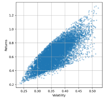
- Creating the minimum Volatility portfolio
min_vol_port = portfolios.iloc[portfolios['Volatility'].idxmin()]
# idxmin() gives us the minimum value in the column specified.
min_vol_port
Returns        0.222657
Volatility     0.235856
AMD weight     0.005248
INTC weight    0.146243
MSI weight     0.819138
NVDA weight    0.029371
Name: 7829, dtype: float64

# plotting the minimum volatility portfolio
plt.subplots(figsize=[7,7])
plt.scatter(portfolios['Volatility'], portfolios['Returns'],marker='o', s=10, alpha=0.3)
plt.scatter(min_vol_port[1], min_vol_port[0], color='r', marker='*', s=500)
plt.xlabel('Volatility',fontsize=14)
plt.ylabel('Returns',fontsize=14)
plt.title("Minimum Volatility Portfolio",fontsize=16)
plt.grid()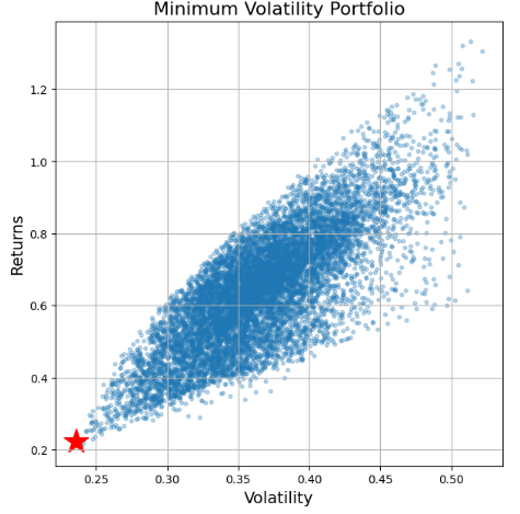
- Finding the optimal portfolio max Sharpe
# Finding the optimal portfolio max Sharpe
rf = 0.01 # risk factor
optimal_risky_port = portfolios.iloc[((portfolios['Returns']-rf)/portfolios['Volatility']).idxmax()]
optimal_risky_port

Returns        1.320434
Volatility     0.507973
AMD weight     0.020084
INTC weight    0.033438
MSI weight     0.068125
NVDA weight    0.878353
Name: 5210, dtype: float64- Plotting both portfolios and the efficient frontier
# Plotting optimal portfolio
plt.subplots(figsize=(8, 8))
plt.scatter(portfolios['Volatility'], portfolios['Returns'],marker='o', s=10, alpha=0.3)
plt.scatter(min_vol_port[1], min_vol_port[0], color='r', marker='*', s=500)
plt.scatter(optimal_risky_port[1], optimal_risky_port[0], color='g', marker='*', s=500)
plt.xlabel('Volatility',fontsize=14)
plt.ylabel('Returns',fontsize=14)
plt.title("Minimum Volatility (Red) vs Optimal Risky (Green) Portfolio",fontsize=14)
plt.grid()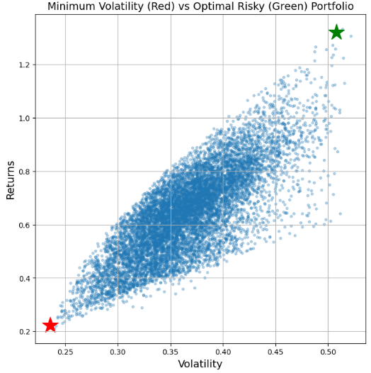
Monte Carlo vs SciPy 2Y MPO
- In this section, we will focus on the MPO-based return and risk of our 2Y tech stock portfolio. By implementing both SciPy Opt and the Monte Carlo Method, we can create a more accurate optimization process compared to traditional methods.
# Load Packages
import numpy as np
import pandas as pd
import matplotlib.pyplot as plt
import plotly.express as px
import pandas_datareader as web
from datetime import datetime as dt, timedelta as td

end = dt.today()
start = end - td(days=2*365)

#option 1
stocks = ['NVDA', 'INTC', 'AMD', 'MSI','^GSPC']
#option 2
stocks = ['NVDA', 'INTC', 'AMD', 'MSI']

# Fetch the data
import yfinance as yf
df = yf.download(stocks,start=start,end=end)['Adj Close']- Plotting the normalized stock prices scaled by 100
px.line(df * 100 / df.iloc[0]) #cf. Stock Returns vs Benchmark- Plotting the daily percentage changes
ret_port = df.pct_change()
px.line(ret_port) #cf. Stock Returns vs Benchmark- Plotting the stock cumulative return
cumretport = (1 + ret_port).cumprod() - 1
px.line(cumretport*100) #cf. Stock Returns vs Benchmarkprint(log_ret.mean()) # option 1
Ticker
AMD 0.001018
INTC -0.000502
MSI 0.000876
NVDA 0.002727
^GSPC 0.000302
dtype: float64- Calculating the expected return and volatility for 1k random portfolios (cf. option 2)
np.random.seed(1)
# Weight each security
weights = np.random.random((4,1))
# normalize it, so that some is one
weights /= np.sum(weights)
print(f'Normalized Weights : {weights.flatten()}')

# We generally do log return instead of return
log_ret = np.log(df / df.shift(1))
log_ret

# Expected return (weighted sum of mean returns). Mult by 252 as we always do annual calculation and year has 252 business days
exp_ret = log_ret.mean()[:-1].dot(weights)*252
print(f'\nExpected return of the portfolio is : {exp_ret[0]}')

# Exp Volatility (Risk)
exp_vol = np.sqrt(weights.T.dot(252*log_ret.cov().dot(weights)))
print(f'\nVolatility of the portfolio: {exp_vol[0][0]}')

# Sharpe ratio
sr = exp_ret / exp_vol
print(f'\nSharpe ratio of the portfolio: {sr[0][0]}')

Normalized Weights : [2.89640161e-01 5.00297106e-01 7.94383512e-05 2.09983296e-01]

# number of simulations
n = 1000

port_weights = np.zeros(shape=(n,len(df.columns)))
port_volatility = np.zeros(n)
port_sr = np.zeros(n)
port_return = np.zeros(n)

num_securities = len(df.columns)
# num_securities
for i in range(n):
    # Weight each security
    weights = np.random.random(4)
    # normalize it, so that some is one
    weights /= np.sum(weights)
    port_weights[i,:] = weights
    #     print(f'Normalized Weights : {weights.flatten()}')

    # Expected return (weighted sum of mean returns). Mult by 252 as we always do annual calculation and year has 252 business days
    exp_ret = log_ret.mean().dot(weights)*252
    port_return[i] = exp_ret
#     print(f'\nExpected return is : {exp_ret[0]}')

    # Exp Volatility (Risk)
    exp_vol = np.sqrt(weights.T.dot(252*log_ret.cov().dot(weights)))
    port_volatility[i] = exp_vol
#     print(f'\nVolatility : {exp_vol[0][0]}')

    # Sharpe ratio
    sr = exp_ret / exp_vol
    port_sr[i] = sr
#     print(f'\nSharpe ratio : {sr[0][0]}')
- Finding the return and volatility at max Sharpe Ratio (SR)
# Index of max Sharpe Ratio
max_sr = port_sr.max()
ind = port_sr.argmax()
# Return and Volatility at Max SR
max_sr_ret = port_return[ind]
max_sr_vol = port_volatility[ind]- Plotting the efficient frontier and the max SR portfolio
plt.figure(figsize=(10,6))
plt.scatter(port_volatility,port_return,c=port_sr, cmap='plasma')
plt.colorbar(label='Sharpe Ratio')
plt.xlabel('Volatility', fontsize=15)
plt.ylabel('Return', fontsize=15)
plt.title('Efficient Frontier (Bullet Plot)', fontsize=15)
plt.scatter(max_sr_vol, max_sr_ret, c='blue', s=150, edgecolors='red', marker='o', label='Max \
Sharpe Ratio Portfolio')
plt.legend();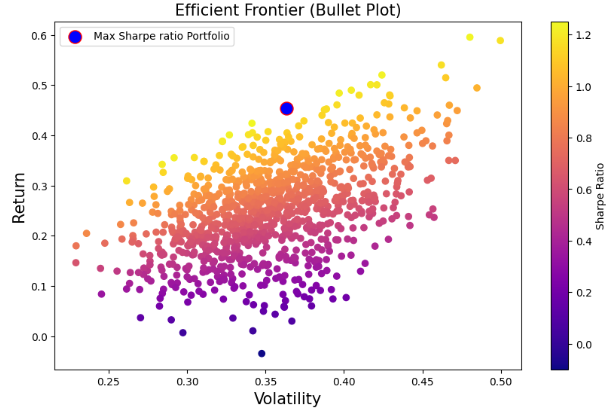
- Optimized portfolio weights, expected returns and volatility
for weight, stock in zip(port_weights[ind],stocks):
    print(f'{round(weight * 100, 2)} % of {stock} should be bought.')

# best portfolio return option 2
print(f'\nMarkowitz optimal portfolio return is : {round(max_sr_ret * 100, 2)}% with volatility \
{max_sr_vol}')

5.69 % of NVDA should be bought.
1.35 % of INTC should be bought.
38.94 % of AMD should be bought.
54.02 % of MSI should be bought.

Markowitz optimal portfolio return is : 45.45% with volatility 0.3632750947781604- Using SciPy to get the max of Sharpe Ratio
#SciPy to get the max of Sharpe Ratio
from scipy import optimize
log_mean = log_ret.mean() * 252
cov = log_ret.cov() * 252

# Some helper functions
def get_ret_vol_sr(weights):
    weights = np.array(weights)
    ret = log_mean.dot(weights)
    vol = np.sqrt(weights.T.dot(cov.dot(weights)))
    sr = ret / vol
    return np.array([ret, vol, sr])

# Negate Sharpe ratio as we need to max it but Scipy minimize the given function
def neg_sr(weights):
    return get_ret_vol_sr(weights)[-1] * -1

# check sum of weights
def check_sum(weights):
    return np.sum(weights) - 1

# Constraints for the optimization problem
cons = {'type':'eq','fun':check_sum}
# bounds on weights
bounds = ((0,1),(0,1),(0,1),(0,1))
# initial guess for optimization to start with
init_guess = [.25 for _ in range(4)]


# Call minimizer
opt_results = optimize.minimize(neg_sr, init_guess, constraints=cons, bounds=bounds, method='SLSQP')

optimal_weights = opt_results.x
# optimal_weights
for st, i in zip(stocks,optimal_weights):
    print(f'Stock {st} has weight {np.round(i*100,2)} %')

Stock NVDA has weight 0.0 %
Stock INTC has weight 0.0 %
Stock AMD has weight 47.28 %
Stock MSI has weight 52.72 %

#Monte Carlo weights

mc_weights = port_weights[ind]
for st, i in zip(stocks,mc_weights):
    print(f'Stock {st} has weight {np.round(i*100,2)} %')

Stock NVDA has weight 5.69 %
Stock INTC has weight 1.35 %
Stock AMD has weight 38.94 %
Stock MSI has weight 54.02 %

# Comparing two results we see that we get very close results
(optimal_weights - mc_weights)

array([-0.05690935, -0.01352879, 0.08342671, -0.01298856])- Comparing expected returns and volatility
get_ret_vol_sr(optimal_weights), get_ret_vol_sr(mc_weights)

print('For a given portfolio we have: (Using SciPy optimizer)\n \n')
for i, j in enumerate('Return Volatility SharpeRatio'.split()):
    print(f'{j} is : {get_ret_vol_sr(optimal_weights)[i]}\n')

print('For a given portfolio we have: (Using Monte Carlo)\n \n')
for i, j in enumerate('Return Volatility SharpeRatio'.split()):
    print(f'{j} is : {get_ret_vol_sr(mc_weights)[i]}\n')

For a given portfolio we have: (Using SciPy optimizer)

Return is : 0.45084758839098316

Volatility is : 0.34220896907233184

SharpeRatio is : 1.3174628052945294

For a given portfolio we have: (Using Monte Carlo)

Return is : 0.45447440930271593

Volatility is : 0.3632750947781604

SharpeRatio is : 1.2510475279904554- Plotting the efficient frontier curve vs max SR portfolio
#Frontier curve
#Best return for given volatility or vice versa.
frontier_y = np.linspace(port_return.min(), port_return.max(), 100)
frontier_vol = []

def minimize_vol(weights):
    return get_ret_vol_sr(weights)[1]

for possible_ret in frontier_y:
    cons = ({'type':'eq','fun':check_sum},
            {'type':'eq','fun':lambda w:get_ret_vol_sr(w)[0] - possible_ret})
    result = optimize.minimize(minimize_vol, init_guess, method='SLSQP', constraints=cons, bounds=bounds)
    frontier_vol.append(result['fun'])

plt.figure(figsize=(10,6))
plt.scatter(port_volatility,port_return,c=port_sr, cmap='plasma')
plt.colorbar(label='Sharpe Ratio')
plt.xlabel('Volatility', fontsize=15)
plt.ylabel('Return', fontsize=15)
plt.title('Efficient Frontier', fontsize=15)
plt.scatter(max_sr_vol, max_sr_ret, c='blue', s=150, edgecolors='red', marker='o')

plt.plot(frontier_vol, frontier_y, c='magenta', ls='--', lw=3, label='Efficient Frontier')
plt.legend();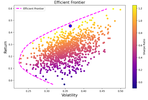
Quantstats Portfolio Report Before MPO
- We employ Quantstats to understand portfolio performance better by examining in-depth analytics and risk metrics vs ^GSPC.
- Our initial portfolio consists of 4 tech stocks (option 2) with equal weights 0.25, viz.
weights = [0.25, 0.25, 0.25, 0.25] # Defining weights for each stock
portfolio = df['NVDA']*weights[0] + df['AMD']*weights[1] + df['INTC']*weights[2] + df['MSI']*weights[3] # Creating portfolio multiplying each stock for its respective weight
portfolio # Portfolio before MPO

Date
2022-04-19    148.027820
2022-04-20    146.227382
2022-04-21    140.810877
2022-04-22    136.540077
2022-04-25    138.295864
                 ...
2024-04-12    356.159995
2024-04-15    348.805001
2024-04-16    353.495004
2024-04-17    342.639997
2024-04-18    347.843740
Length: 503, dtype: float64- Plotting the full portfolio report vs ^GSPC benchmark
qs.reports.full(portfolio, benchmark = df['^GSPC'])

Performance Metrics

                           Benchmark    Strategy
-------------------------  -----------  ----------
Start Period               2022-04-20   2022-04-20
End Period                 2024-04-18   2024-04-18
Risk-Free Rate             0.0%         0.0%
Time in Market             100.0%       100.0%

Cumulative Return          13.12%       134.99%
CAGR﹪                     4.35%        34.36%

Sharpe                     0.43         1.41
Prob. Sharpe Ratio         72.72%       97.91%
Smart Sharpe               0.42         1.37
Sortino                    0.61         2.26
Smart Sortino              0.6          2.19
Sortino/√2                 0.43         1.6
Smart Sortino/√2           0.42         1.55
Omega                      1.27         1.27

Max Drawdown               -19.79%      -31.21%
Longest DD Days            447          287
Volatility (ann.)          18.32%       34.63%
R^2                        0.64         0.64
Information Ratio          0.11         0.11
Calmar                     0.22         1.1
Skew                       -0.11        0.55
Kurtosis                   2.03         2.88

Expected Daily %           0.02%        0.17%
Expected Monthly %         0.49%        3.48%
Expected Yearly %          4.2%         32.95%
Kelly Criterion            1.98%        12.12%
Risk of Ruin               0.0%         0.0%
Daily Value-at-Risk        -1.87%       -3.39%
Expected Shortfall (cVaR)  -1.87%       -3.39%

Max Consecutive Wins       8            11
Max Consecutive Losses     6            7
Gain/Pain Ratio            0.08         0.27
Gain/Pain (1M)             0.31         1.27

Payoff Ratio               1.03         1.16
Profit Factor              1.08         1.27
Common Sense Ratio         1.24         1.6
CPC Index                  0.56         0.78
Tail Ratio                 1.15         1.26
Outlier Win Ratio          4.82         2.45
Outlier Loss Ratio         5.33         2.88

MTD                        -3.93%       -6.19%
3M                         6.51%        28.51%
6M                         15.42%       60.21%
YTD                        5.83%        38.46%
1Y                         21.59%       104.94%
3Y (ann.)                  4.35%        34.36%
5Y (ann.)                  4.35%        34.36%
10Y (ann.)                 4.35%        34.36%
All-time (ann.)            4.35%        34.36%

Best Day                   5.54%        11.53%
Worst Day                  -4.32%       -6.06%
Best Month                 9.11%        18.49%
Worst Month                -9.34%       -14.91%
Best Year                  24.23%       104.95%
Worst Year                 -13.96%      -17.19%

Avg. Drawdown              -2.28%       -3.72%
Avg. Drawdown Days         30           18
Recovery Factor            0.79         3.12
Ulcer Index                0.09         0.1
Serenity Index             0.13         1.12

Avg. Up Month              4.66%        11.94%
Avg. Down Month            -5.78%       -9.36%
Win Days %                 50.2%        52.79%
Win Month %                60.0%        64.0%
Win Quarter %              55.56%       55.56%
Win Year %                 66.67%       66.67%

Beta                       -            1.52
Alpha                      -            0.37
Correlation                -            80.15%
Treynor Ratio              -            89.09%
None
Worst 5 Drawdowns
Start Valley End Days Max Drawdown 99% Max Drawdown
1 2022-04-21 2022-10-14 2023-02-01 287 -31.213813 -28.614034
2 2023-09-01 2023-10-26 2023-11-07 68 -12.313689 -11.760164
3 2024-03-26 2024-04-17 2024-04-18 24 -9.736568 -8.365719
4 2023-07-19 2023-08-11 2023-08-30 43 -8.844754 -7.638776
5 2023-02-15 2023-02-22 2023-03-07 21 -6.694283 -6.039259

Strategy Visualization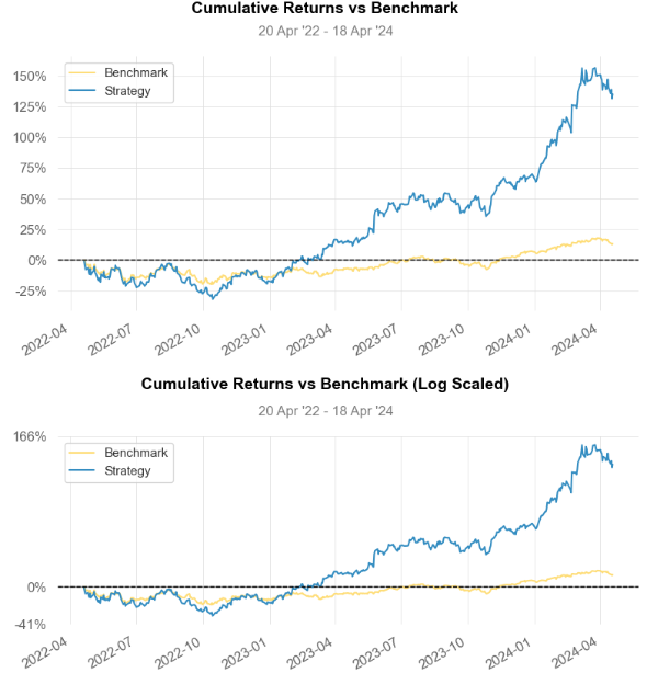
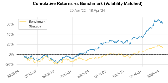
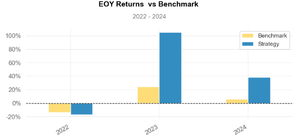
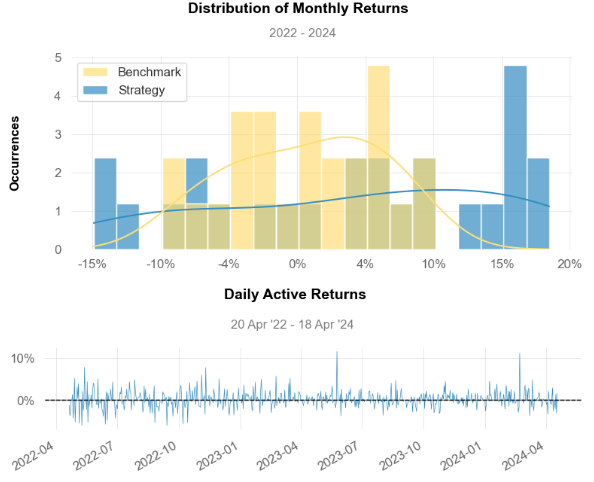
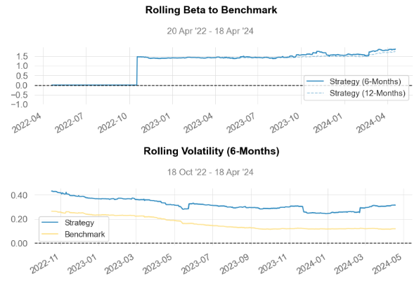
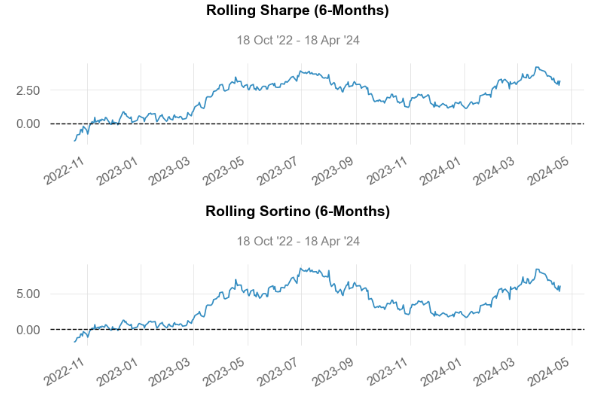
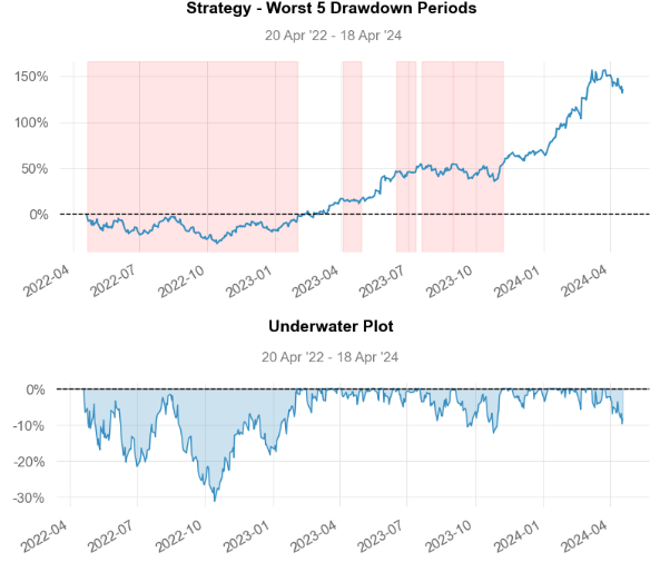
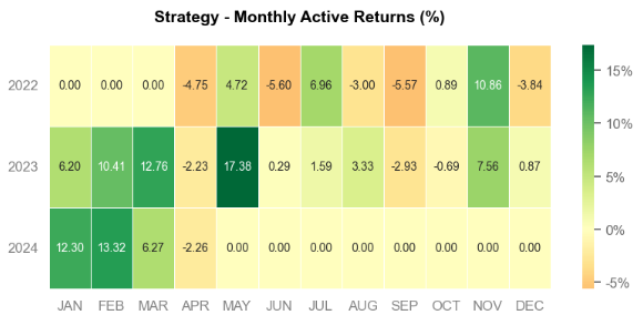
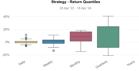
Quantstats Portfolio Report After MPO
- Our updated portfolio after MPO consists of 4 tech stocks (option 2) with optimized weights, viz.
#Optimized max Sharpe Ratio SciPy
weights = [0.06, 0.39, 0.01, 0.54] # Defining weights for each stock
portfolio = df['NVDA']*weights[0] + df['AMD']*weights[1] + df['INTC']*weights[2] + df['MSI']*weights[3] # Creating portfolio multiplying each stock for its respective weight
portfolio # Portfolio after MPO

Date
2022-04-19    174.796358
2022-04-20    174.686317
2022-04-21    170.144846
2022-04-22    164.859244
2022-04-25    166.153715
                 ...
2024-04-12    302.605097
2024-04-15    297.321696
2024-04-16    300.220396
2024-04-17    294.721005
2024-04-18    296.741143
Length: 503, dtype: float64- Plotting the optimized portfolio report vs ^GSPC benchmark
qs.reports.full(portfolio, benchmark = df['^GSPC'])

Performance Metrics

                           Benchmark    Strategy
-------------------------  -----------  ----------
Start Period               2022-04-20   2022-04-20
End Period                 2024-04-18   2024-04-18
Risk-Free Rate             0.0%         0.0%
Time in Market             100.0%       100.0%

Cumulative Return          13.12%       69.76%
CAGR﹪                     4.35%        20.08%

Sharpe                     0.43         1.14
Prob. Sharpe Ratio         72.72%       94.8%
Smart Sharpe               0.4          1.07
Sortino                    0.61         1.77
Smart Sortino              0.58         1.66
Sortino/√2                 0.43         1.25
Smart Sortino/√2           0.41         1.17
Omega                      1.22         1.22

Max Drawdown               -19.79%      -23.87%
Longest DD Days            447          177
Volatility (ann.)          18.32%       26.29%
R^2                        0.66         0.66
Information Ratio          0.09         0.09
Calmar                     0.22         0.84
Skew                       -0.11        0.28
Kurtosis                   2.03         1.91

Expected Daily %           0.02%        0.11%
Expected Monthly %         0.49%        2.14%
Expected Yearly %          4.2%         19.29%
Kelly Criterion            1.14%        9.95%
Risk of Ruin               0.0%         0.0%
Daily Value-at-Risk        -1.87%       -2.61%
Expected Shortfall (cVaR)  -1.87%       -2.61%

Max Consecutive Wins       8            8
Max Consecutive Losses     6            7
Gain/Pain Ratio            0.08         0.22
Gain/Pain (1M)             0.31         1.1

Payoff Ratio               1.02         1.14
Profit Factor              1.08         1.22
Common Sense Ratio         1.24         1.56
CPC Index                  0.55         0.72
Tail Ratio                 1.15         1.28
Outlier Win Ratio          4.23         2.88
Outlier Loss Ratio         4.75         3.39

MTD                        -3.93%       -6.31%
3M                         6.51%        11.03%
6M                         15.42%       32.87%
YTD                        5.83%        15.78%
1Y                         21.59%       43.52%
3Y (ann.)                  4.35%        20.08%
5Y (ann.)                  4.35%        20.08%
10Y (ann.)                 4.35%        20.08%
All-time (ann.)            4.35%        20.08%

Best Day                   5.54%        7.53%
Worst Day                  -4.32%       -5.35%
Best Month                 9.11%        17.09%
Worst Month                -9.34%       -11.76%
Best Year                  24.23%       49.61%
Worst Year                 -13.96%      -2.0%

Avg. Drawdown              -2.28%       -3.14%
Avg. Drawdown Days         30           19
Recovery Factor            0.79         2.51
Ulcer Index                0.09         0.07
Serenity Index             0.13         1.13

Avg. Up Month              4.78%        8.58%
Avg. Down Month            -5.73%       -6.69%
Win Days %                 50.2%        51.99%
Win Month %                60.0%        60.0%
Win Quarter %              55.56%       66.67%
Win Year %                 66.67%       66.67%

Beta                       -            1.16
Alpha                      -            0.21
Correlation                -            80.94%
Treynor Ratio              -            60.06%
None
Worst 5 Drawdowns
Start Valley End Days Max Drawdown 99% Max Drawdown
1 2022-08-17 2022-10-14 2023-02-09 177 -23.867018 -20.927214
2 2022-04-21 2022-06-16 2022-08-01 103 -16.555311 -14.846316
3 2023-07-26 2023-10-27 2023-11-02 100 -9.848466 -9.803296
4 2024-03-08 2024-04-17 2024-04-18 42 -7.452712 -6.818356
5 2023-02-16 2023-02-22 2023-03-15 28 -4.578890 -4.128242
Strategy Visualization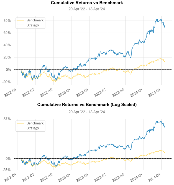
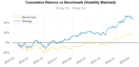
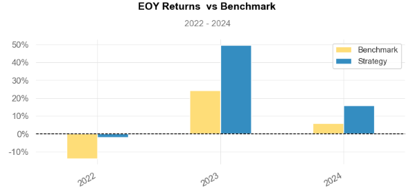
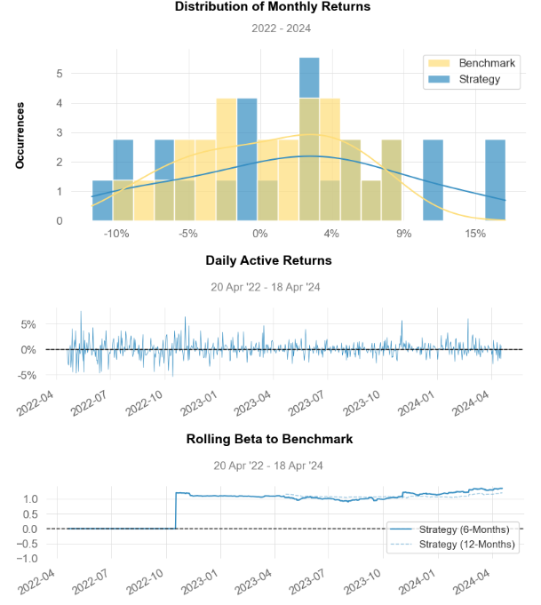
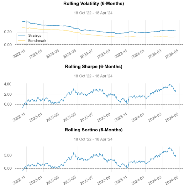
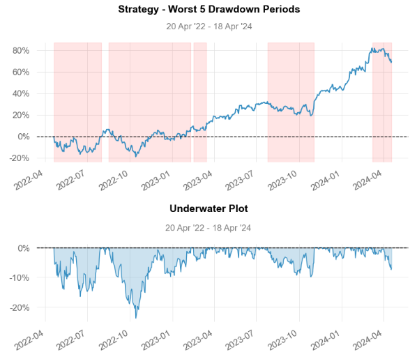
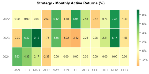
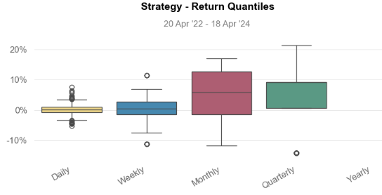
Conclusions
- In this post, we have addressed the challenge of Financial Risk Management (FRM) for Automated Trading (AT) and Investments in Stocks.
- We have implemented and tested state-of-the art FRM tools and techniques in stock AT and investments.
- We have deployed a set of SaaS products to open and close trades according to set rules such as points of price movement in an underlying market. Once the current market conditions match any predetermined criteria, our trading algorithms (algos) can execute a buy or sell order on your behalf.
- As a pilot project, we have used these products to perform robust backtesting, technical/fundamental financial analysis, and stochastic portfolio optimization of 4 tech game-changers (NVDA, AMD, INTC & MSI) vs S&P 500 benchmark.
- Our interactive stock screening and portfolio optimization dashboard can quickly and easily see the asset’s health at a glance and identify areas that require attention. In addition, our fintech KPI visualizations can communicate the risks associated with specific investments.
- Overall, we have looked at AT use-case examples based on best fintech industry practices that set to accelerate the AT market growth in the near future. Factors such as the increasing adoption of numerical optimization and stochastic simulation methods, real-time data analytics, interactive visualizations, and the rising demand for automated trading systems substantiate the great business value of our study.
Explore More
- A Market-Neutral Strategy
- A Comprehensive Analysis of Best Trading Technical Indicators w/ TA-Lib — Tesla ‘23
- Plotly Dash TA Stock Market App
- Returns-Volatility Domain K-Means Clustering and LSTM Anomaly Detection of S&P 500 Stocks
- NVIDIA Returns-Drawdowns MVA & RNN Mean Reversal Trading
- Oracle Monte Carlo Stock Simulations
- NVIDIA Rolling Volatility: GARCH & XGBoost
- IQR-Based Log Price Volatility Ranking of Top 19 Blue Chips
- Multiple-Criteria Technical Analysis of Blue Chips in Python
- Datapane Stock Screener App from Scratch
- Data Visualization in Python — 1. Stock Technical Indicators
- Top 6 Reliability/Risk Engineering Learnings
- JPM Breakouts: Auto ARIMA, FFT, LSTM & Stock Indicators
- Post-SVB Risk Aware Investing
- Applying a Risk-Aware Portfolio Rebalancing Strategy to ETF, Energy, Pharma, and Aerospace/Defense Stocks in 2023
- Portfolio Optimization of 20 Dividend Growth Stocks
- Donchian Channel Trading Systems
- Towards Max(ROI/Risk) Trading
- The Qullamaggie’s TSLA Breakouts for Swing Traders
- Algorithmic Testing Stock Portfolios to Optimize the Risk/Reward Ratio
- Quant Trading using Monte Carlo Predictions and 62 AI-Assisted Trading Technical Indicators (TTI)
- Top 6 Reliability/Risk Engineering Learnings
- Stock Portfolio Risk/Return Optimization
- Risk/Return QC via Portfolio Optimization — Current Positions of The Dividend Breeder
- Portfolio Optimization Risk/Return QC — Positions of Humble Div vs Dividend Glenn
- Risk/Return POA — Dr. Dividend’s Positions
- Bear Market Similarity Analysis using Nasdaq 100 Index Data
- Inflation-Resistant Stocks to Buy
- Basic Stock Price Analysis in Python
- Predicting Trend Reversal in Algorithmic Trading using Stochastic Oscillator in Python
- Bear vs. Bull Portfolio Risk/Return Optimization QC Analysis
- The CodeX-Aroon Auto-Trading Approach — the AAPL Use Case
- DJI Market State Analysis using the Cruz Fitting Algorithm
- Risk-Aware Strategies for DCA Investors
- The $ASML Trading Strategies via the Plotly Stock Market Dashboard
- Python Technical Analysis for BioTech — Get Buy Alerts on ABBV in 2023
Acknowledgements
References
- Data Science for Financial Markets
- Beta of a Stock & CAPM from Scratch
- Algorithmic Trading — Backtesting a strategy in python
- Portfolio Optimization with Python using Efficient Frontier with Practical Examples
- PyroQuant/Portfolio-Optimizer
- Portfolio optimization using Python
- Python for Finance: Portfolio Optimization
- Historical Stock Price Data in Python
- Markowitz Portfolio Optimization in Python/v3
- Portfolio Optimization with Python: using SciPy Optimize & Monte Carlo Method
- ranaroussi/quantstats
Relevant 3rd Party SaaS Platforms
Stock Market Research Updates
- A Weekday Market Research Update
- Towards min(Risk/Reward) — SeekingAlpha August Bear Market Update
- All Eyes on ETFs Sep ‘22
- Zacks Investment Research Update Q4'22
- Stocks to Watch in 2023: MarketBeat Ideas