
NVIDIA Algo-Trading: VaR, Q-Q Plots & Stochastic Simulations

- In this post, we will gain a deeper insight into the latest NVIDIA (NASDAQ: NVDA) stock trends in terms of the Value-at-Risk (VaR), Q-Q probability plots and 1Y Monte-Carlo (MC) simulations of the share price by adapting the risk engineering stock market notebook in Python.
- VaR is a commonly used method for measuring portfolio risk: a negative VaR would imply the portfolio has a high probability of making a profit, e.g. a 1-day 5% VaR of -$1k implies the portfolio has a 95% chance of making more than $1k over the next day.
- Firstly, we will examine how to estimate VaR using MC methods, as explained here.
- Secondly, we will compare the Q-Q plots for normal and student distributions.
- Our ultimate goal is to understand how the NVDA risk is modeled, characterized and quantified.
- Let’s get into details!
Reading Input Data
- Importing key libraries
import numpy
import pandas
import scipy.stats
import matplotlib.pyplot as plt
import requests
from math import floor
from termcolor import colored as cl
import numpy as np
import pandas as pd
plt.style.use("bmh")
%config InlineBackend.figure_formats=["png"]
from yahoofinancials import YahooFinancials
from datetime import datetime- Reading the NVDA historical stock data
def retrieve_stock_data(ticker, start, end):
    json = YahooFinancials(ticker).get_historical_price_data(start, end, "daily")
    df = pandas.DataFrame(columns=["open","close","adjclose"])
    for row in json[ticker]["prices"]:
        date = datetime.fromisoformat(row["formatted_date"])
        df.loc[date] = [row["open"], row["close"], row["adjclose"]]
    df.index.name = "date"
    return df

def get_historical_data(symbol, start_date):
    api_key = 'YOUR API KEY'
    api_url = f'https://api.twelvedata.com/time_series?symbol={symbol}&interval=1day&outputsize=5000&apikey={api_key}'
    raw_df = requests.get(api_url).json()
    df = pd.DataFrame(raw_df['values']).iloc[::-1].set_index('datetime').astype(float)
    df = df[df.index >= start_date]
    df.index = pd.to_datetime(df.index)
    return d

nvd = get_historical_data('NVDA', '2023-01-03')
nvd.tail()

           open      high      low       close     volume
datetime
2024-04-01 902.98999 922.25000 892.03998 903.63000 45244100.0
2024-04-02 884.47998 900.94000 876.20001 894.52002 43306400.0
2024-04-03 884.84003 903.73999 884.00000 889.64001 36845000.0
2024-04-04 904.06000 906.34003 858.79999 859.04999 43496500.0
2024-04-05 868.65997 884.81000 859.26001 880.08002 39885700.0- Plotting the NVIDIA stock data
fig = plt.figure()
fig.set_size_inches(10,3)
nvd["close"].plot()
plt.title("NVDA stock", weight="bold");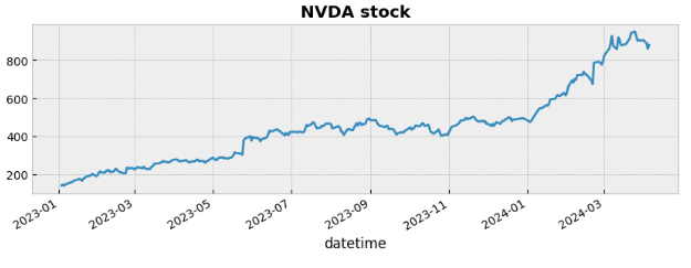
- Plotting the NVDA daily returns
fig = plt.figure()
fig.set_size_inches(10,3)
nvd["close"].pct_change().plot()
plt.title("NVDA daily returns", weight="bold");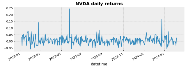
- Plotting the histogram of NVDA daily returns and printing std
nvd["close"].pct_change().hist(bins=50, density=True, histtype="stepfilled", alpha=0.5)
plt.title("Histogram of NVDA daily returns", weight="bold")
nvd["close"].pct_change().std()
0.030739970163706058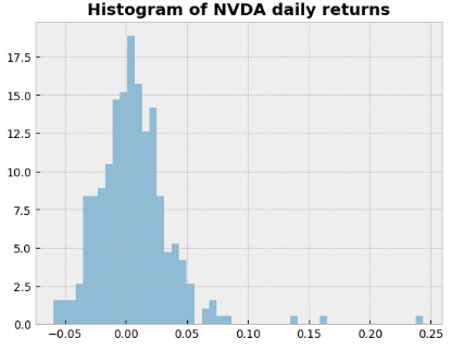
Q-Q Plots of Daily Returns
- Let’s look at the Q-Q plot to assess if a dataset came from some theoretical distribution such as a normal/student.
- Plotting the normal probability plot of NVDA daily returns
Q = nvd["close"].pct_change().dropna()
scipy.stats.probplot(Q, dist=scipy.stats.norm, plot=plt.figure().add_subplot(111))
plt.title("Normal probability plot of NVDA daily returns", weight="bold");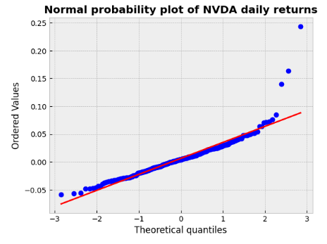
- Here, the 0.95 quantile, or 95th percentile, is about 1.64. 95 % of the data lie below 1.64. This plot shows that the dataset does look a lot like a normal distribution with the 95% confidence.
- Plotting the Student probability plot of NVDA daily returns
tdf, tmean, tsigma = scipy.stats.t.fit(Q)
scipy.stats.probplot(Q, dist=scipy.stats.t, sparams=(tdf, tmean, tsigma), plot=plt.figure().add_subplot(111))
plt.title("Student probability plot of NVDA daily returns", weight="bold");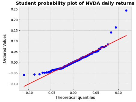
- The above graph plots the quantiles of a data sample against the theoretical quantiles of a Student’s t-distribution. Student’s t distribution does not seem to fit better than normal distribution (look in particular at the tails of the distribution).
VaR & 1Y MC Simulations
- Calculating the daily change in NVDA (%).
- Calculating analytic quantiles by curve fitting to historical data. Here, we use Student’s t distribution (we checked above that it represents daily returns relatively well)
support = numpy.linspace(returns.min(), returns.max(), 100)
returns.hist(bins=40, density=True, histtype="stepfilled", alpha=0.5);
plt.plot(support, scipy.stats.t.pdf(support, loc=tmean, scale=tsigma, df=tdf), "r-")
plt.title("Daily change in NVDA (%)", weight="bold");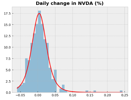
- Printing the 0.05 empirical quantile of daily returns
returns.quantile(0.05)
-0.034305503007941954- The 0.05 empirical quantile of daily returns is at -0.034. That means that with 95% confidence, our worst daily loss will not exceed 3.4%. If we have a $1 M investment, our one-day 5% VaR is 0.034 * $1 M = $34 k.
- Printing the drift (average growth rate) and volatility parameters
print (mean,sigma)
0.006232409253778064 0.030739970163706058- Implementing the method
norm.ppf()that takes a percentage and returns a standard deviation multiplier for what value that percentage occurs at. It returns a 95% significance interval for a one-tail test on a standard normal distribution (i.e. a special case of the normal distribution where the mean is 0 and the standard deviation is 1)
scipy.stats.norm.ppf(0.05, mean, sigma)
-0.04433034216237391
Our analytic 0.05 quantile is at -0.0443, so with 95% confidence, our worst daily loss will not exceed 4.43%. For a $1 M investment, 1-day VaR is 0.0443 * $1 M ~ $44 k.
- Defining input parameters of the geometric Brownian motion
days = 300   # time horizon
dt = 1/float(days)
sigma = 0.030739970163706058 # volatility
mu = 0.006232409253778064  # drift (average growth rate)
startprice=880.08
The function random_walk simulates one stock market evolution, and returns the price evolution as an array. It simulates geometric Brownian motion using pseudorandom numbers drawn from the aforementioned normal distribution
def random_walk(startprice):
    price = numpy.zeros(days)
    shock = numpy.zeros(days)
    price[0] = startprice
    for i in range(1, days):
        shock[i] = numpy.random.normal(loc=mu * dt, scale=sigma * numpy.sqrt(dt))
        price[i] = max(0, price[i-1] + shock[i] * price[i-1])
return price- Plotting 300 random walks, starting from an initial stock price of $880.08, for a duration of 300 days.
plt.figure(figsize=(9,4))
for run in range(300):
    plt.plot(random_walk(880.08))
plt.xlabel("Days")
plt.ylabel("Price USD");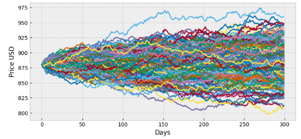
- Final price is spread out between $800 (our portfolio has lost value) to almost $975. We can see graphically that the expectation (mean outcome) is a profit; this is due to the fact that the drift in our random walk (parameter mu) is positive.
- Run a MC simulation of random walks to obtain the PDF of the final price, including quantile measures for VaR
runs = 10000
simulations = numpy.zeros(runs)
for run in range(runs):
    simulations[run] = random_walk(startprice)[days-1]
q = numpy.percentile(simulations, 1)
plt.hist(simulations, density=True, bins=30, histtype="stepfilled", alpha=0.5)
plt.figtext(0.6, 0.8, "Start price: $880.08")
plt.figtext(0.6, 0.7, "Mean final price: ${:.3}".format(simulations.mean()))
plt.figtext(0.6, 0.6, "VaR(0.99): ${:.3}".format(10 - q))
plt.figtext(0.15, 0.6, "q(0.99): ${:.3}".format(q))
plt.axvline(x=q, linewidth=4, color="r")
plt.title("Final price distribution after {} days".format(days), weight="bold");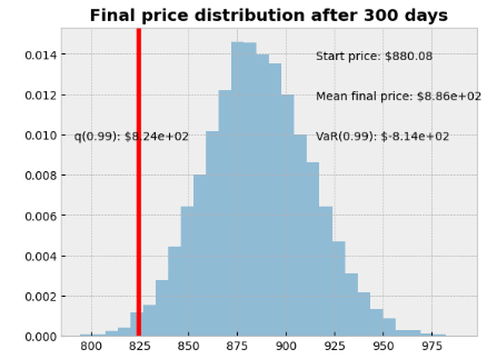
- We have looked at the 1% empirical quantile of the final price distribution to estimate VaR, which is $814 for a $880.08 investment. It is defined as the maximum dollar amount expected to be lost over a given time horizon, at a pre-defined confidence level.
Conclusions
- We have examined the NVDA historical stock price in terms of Q-Q and VaR of daily returns.
- VAR has been defined as the loss level that will not be exceeded with a certain confidence level during a certain period of time.
- Key VaR elements are the specified amount of loss in percentage, time period, and confidence interval.
- Our VaR analysis has been substantiated by 10k random walks for a duration of 300 days.
- This study supports the NVDA VaR Peers Comparison relative to other trading indicators.
- This study can be used by different financial institutions to assess the profitability and risk of NVDA, and allocate risk based on VaR.
Explore More
- Top 6 Reliability/Risk Engineering Learnings
- Oracle Monte Carlo Stock Simulations
- NVIDIA Rolling Volatility: GARCH & XGBoost
- NVIDIA Returns-Drawdowns MVA & RNN Mean Reversal Trading
- IQR-Based Log Price Volatility Ranking of Top 19 Blue Chips
References
- Stock market trends and Value at Risk
- Understanding QQ Plots
- Predicting Stock Prices using Monte Carlo Simulation
- Predicting Stock Movements with Monte Carlo Simulation: A Powerful Approach for Investors
- Returns-Volatility Domain K-Means Clustering and LSTM Anomaly Detection of S&P 500 Stocks


