The Power of Conditional Value-at-Risk (CVaR). Mastering Risk Management in Python

In today’s volatile markets, investors are looking for better ways to manage risk. Value at Risk (VaR) is a commonly used method for measuring portfolio risk. However, Conditional Value at Risk (CVaR), also known as Expected Shortfall, is gaining popularity as a more comprehensive risk measure that takes into account the tail risk of an investment portfolio.

In this article, we will explore the advantages of using CVaR over VaR for portfolio risk management, and provide a step-by-step guide on how to calculate and visualize CVaR using Python.

To begin, we'll import the necessary libraries:

import pandas as pd
import numpy as np
import yfinance as yf
from scipy.stats import norm

Download Data

The first step is to extract the tickers of the S&P 100 components from Wikipedia using pandas:

# Get SP100 tickers
url = 'https://en.wikipedia.org/wiki/S%26P_100'
tables = pd.read_html(url)
sp100 = tables[2]
tickers = sp100['Symbol'].tolist()

We'll use the yfinance library to download the stock data for the tickers:

# Download tickers ohlc
df = yf.download(tickers, start='2015-01-01', end='2023-03-14')

CVaR Analysis

The first step is to calculate the daily returns for each stock:

# Calculate Returns
returns = df['Adj Close'].pct_change().dropna()

Now, let's define a function to calculate the CVaR:

# CVaR Function
def cvar(returns, alpha=0.05):
    var = norm.ppf(alpha) * returns.std()
    returns_less_than_var = returns[returns < -var]
    return -returns_less_than_var.mean()

The function takes in the returns and alpha, where alpha is the confidence level. We'll set alpha to 0.05, which corresponds to a 95% confidence level.

CVaR is derived by taking a weighted average of the “extreme” losses in the tail of the distribution of possible returns, beyond the VaR cutoff point. Conditional value at risk is used in portfolio optimization for effective risk management.

We'll now calculate the CVaR for each stock and sort them in descending order:

cvar_dict = {}

# Calculate CVaR for each ticker
for ticker in tickers:
    cvar_dict[ticker] = cvar(returns[ticker])

cvar_df = pd.DataFrame.from_dict(cvar_dict, orient='index', columns=['CVaR'])
cvar_df = cvar_df.sort_values(by='CVaR', ascending=False)
print(cvar_df.head())

The output should be a sorted DataFrame showing the top 5 stocks with the highest CVaR values.

          CVaR
TSLA  0.002707
GE    0.002702
GM    0.002366
AMD   0.002327
PYPL  0.002167

We can plot a histogram of the CVaR values to visualize the distribution:

# Visualize CVaR distribution
cvar_df.hist(bins=20, figsize=(12, 6), color='lightblue')
plt.xlabel('CVaR')
plt.ylabel('Frequency')
plt.title('Distribution of CVaR Values')
plt.show() 

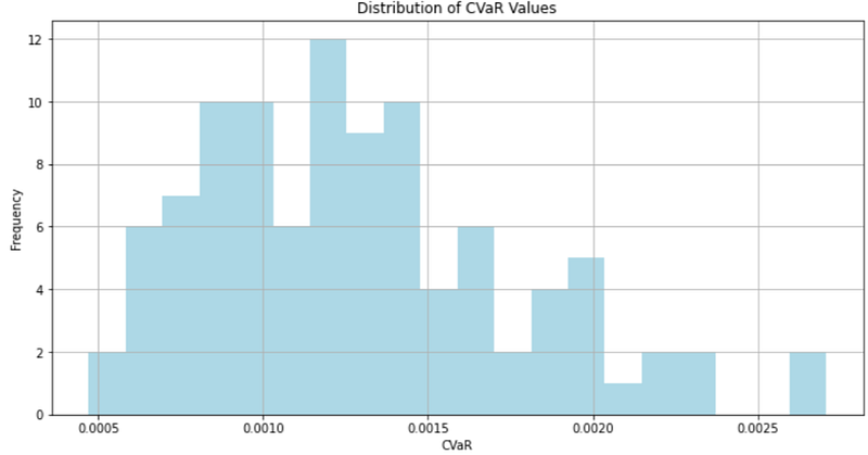
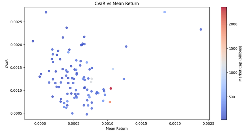
Now that we have calculated the CVaR for each stock in the S&P 100 and plotted a histogram to visualize the distribution, let's explore the relationship between CVaR and mean return by market capitalization.

To do this, we first need to extract the market capitalization for each stock. We can use the fast_info method from the yfinance library to obtain this information.

# calculate CVaR for each stock
cvar_dict = {}
for ticker in tickers:
    cvar_dict[ticker] = cvar(returns[ticker])
cvar_df = pd.DataFrame.from_dict(cvar_dict, orient='index', columns=['CVaR'])

# merge with mean returns
mean_returns = returns.mean().to_frame(name='Mean Return')
merged_df = pd.merge(mean_returns, cvar_df, left_index=True, right_index=True)

# extract market caps
market_caps_dict = {}
for ticker in tickers:
    try:
        ticker_info = yf.Ticker(ticker).fast_info
        market_cap = ticker_info['marketCap'] / 1000000000 # convert to billions
        market_caps_dict[ticker] = market_cap
    except:
        print(f"Data not available for {ticker}")
        market_caps_dict[ticker] = None # set to None if data not available

market_caps = pd.Series(market_caps_dict, name='Market Cap')
market_caps = market_caps.sort_index()
merged_df = pd.merge(merged_df, market_caps.to_frame(), left_index=True, right_index=True)

# plot scatter plot with color gradient
plt.scatter(merged_df['Mean Return'], merged_df['CVaR'], c=merged_df['Market Cap'], alpha=0.8, cmap='coolwarm')
plt.xlabel('Mean Return')
plt.ylabel('CVaR')
plt.title('CVaR vs Mean Return')
plt.colorbar(label='Market Cap (billions)')
plt.show()

In above code, we extract the market capitalization for each stock using the fast_info method from the yfinance library. We then create a dictionary to store the market capitalization for each stock. If the data is not available for a particular stock, we set the market capitalization to None. This dictionary is converted into a Series object and sort it by ticker symbol. We then merge the mean_returns, cvar_df, and market_caps dataframes into a single dataframe merged_df.

Finally, we create a scatter plot of CVaR vs Mean Returns, with the market capitalization represented by a color gradient. This plot allows us to see how the CVaR and mean return of each stock in the S&P 100 are related to its market capitalization. We can observe whether stocks with higher market capitalizations tend to have lower CVaRs or higher mean returns, and vice versa.

Portfolio CVaR & VaR Comparison

Calculating VaR and CVaR for a portfolio is an essential part of risk management. In this section, we will learn how to calculate VaR and CVaR for a portfolio using two new functions with portfolio parameters. We will also plot the portfolio returns and observe the historical VaR and CVaR.

First, let’s define the methods that we will be using. The value_at_risk function calculates the VaR for a portfolio given the value invested, returns, weights and alpha. It calculates the portfolio mean and standard deviation, then uses the inverse of the standard normal cumulative distribution function to get the z-score. Finally, it calculates the VaR using the z-score, standard deviation and mean.

The cvar function calculates the CVaR for a portfolio given the value invested, returns, weights and alpha. It first calculates the portfolio mean and the alpha quantile of the portfolio returns. Then, it selects the returns that are less than the alpha quantile and calculates the CVaR using the selected returns and the portfolio mean.

# Portfolio VaR
def value_at_risk(value_invested, returns, weights, alpha=0.05):
    portfolio_returns = returns.fillna(0.0).dot(weights)
    portfolio_std = portfolio_returns.std()
    portfolio_mean = portfolio_returns.mean()

    z_score = norm.ppf(alpha)
    VaR = -(portfolio_mean - z_score * portfolio_std) * value_invested

    return VaR

# Portfolio CVaR
def cvar(value_invested, returns, weights, alpha=0.05):
    portfolio_returns = returns.fillna(0.0).dot(weights)
    portfolio_mean = portfolio_returns.mean()
    portfolio_var = portfolio_returns.quantile(alpha)
    mask = portfolio_returns < portfolio_var
    portfolio_cvar = -value_invested * (portfolio_mean - portfolio_returns[mask].mean())

    return portfolio_cvar

Once we have defined these functions, we can proceed to calculate VaR and CVaR for our portfolio. We first specify the number of lookback days and the value invested. As an example we set the weights of each stock to be equal. We calculate the portfolio returns for the last 500 days and then calculate the VaR and CVaR using the value_at_risk and cvar functions.

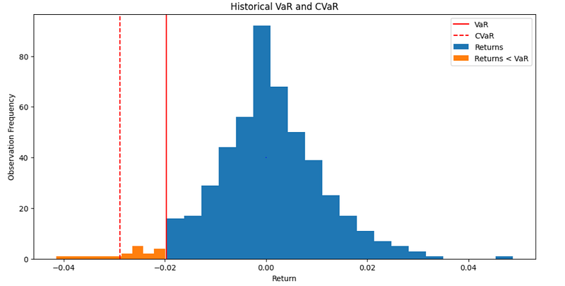
Finally, we create a histogram of the portfolio’s returns and differentiate between returns greater than and less than the VaR return. The solid red line represents VaR and the dashed red line represents CVaR.

# Portfolio parameters
lookback_days = 500
value_invested = 10000 
weights = pd.Series(1.0/len(tickers), index=tickers)

# Portfolio Returns
portfolio_returns = returns.fillna(0.0).iloc[-lookback_days:].dot(weights)

# Portfolio VaR & CVaR
portfolio_VaR = value_at_risk(value_invested, returns, weights, alpha=0.05)
portfolio_VaR_return = portfolio_VaR / value_invested

portfolio_CVaR = cvar(value_invested, returns, weights, alpha=0.05)
portfolio_CVaR_return = portfolio_CVaR / value_invested

# Plot VaR & CVaR histogram
plt.figure(figsize=(12, 6), dpi=100)
plt.hist(portfolio_returns[portfolio_returns > portfolio_VaR_return], bins=20)
plt.hist(portfolio_returns[portfolio_returns < portfolio_VaR_return], bins=10)
plt.axvline(portfolio_VaR_return, color='red', linestyle='solid')
plt.axvline(portfolio_CVaR_return, color='red', linestyle='dashed')
plt.legend(['VaR', 'CVaR', 'Returns', 'Returns < VaR'])
plt.title('Historical VaR and CVaR')
plt.xlabel('Return')
plt.ylabel('Observation Frequency')

VaR identifies the negative return at the 5th percentile, while CVaR considers all the losses to the left of VaR (i.e., the orange bars), including the large negative return. Since returns are not distributed normally, CVaR is better suited for capturing the risk.

Conclusion

In conclusion, this article has shown how CVaR can provide a more complete and robust risk measurement compared to VaR. While VaR only considers the magnitude of the worst-case scenario, CVaR takes into account the entire tail of the distribution, providing a more accurate representation of potential losses.

We have demonstrated how to calculate and visualize CVaR using historical data and how it can be applied to portfolio management. By incorporating CVaR into investment decision-making, investors can have a more comprehensive understanding of the potential risks involved and make more informed choices to achieve their financial goals.

Become a Medium member today and enjoy unlimited access to thousands of Python guides and Data Science articles! For just $5 a month, you’ll have access to exclusive content and support me as a writer. Sign up now using my link and I’ll earn a small commission at no extra cost to you.