Algo-Trading NVIDIA with Donchian Channels

NVIDIA (NASDAQ: NVDA) has come to dominate the market for chips used in AI-powered platforms, bringing its market capitalization to more than $2.28 trillion, an increase of over $1 trillion from its value at the beginning of the year.
TradingView: Nvidia’s earnings for the current year have risen by 3.1% over the past month to $23.84. Furthermore, Nvidia is projected to experience a significant EPS growth of 84% this year.
Indeed, NVDA stock smashed through earnings expectations, sending its shares — and the shares of adjacent AI stocks — rocketing higher. But bull runs don’t last forever. Therefore, it’s always wise to keep an eye on the exit strategy.
The objective of this post is further validate the current NVDA technicals, trading ideas and analyst recommendations using Donchian channels.
Donchian Channels (DC) are a technical indicator that seeks to identify bullish and bearish extremes that favor reversals, higher and lower breakouts, breakdowns, and other emerging trends.
Why DC: Combining SMA/EMA, volume indicators, and MACD with DC can lead to a more complete picture of the market for an asset.
Method: We take on board the algo-trading algorithm in Python that consists of the following steps (cf. Strategy 1: Donchian Middle Value Cross-Over):
Step 1: Reading the NVDA stock historical data using yfinance
Step 2: Create a visualization of the Donchian Channel using matplotlib
Step 3: Implementing the Donchian Middle Value Cross-Over Strategy 1
Step 4: Compare the cumulative returns and relevant stock Risk/Return KPIs (total/annual ROI, annual volatility, Sortino/Sharpe ratio, max drawdowns, and max drawdown durations) of Strategy 1 vs Buy-and-Hold default.
Let’s delve into the implementation details in Jupyter Notebook!
Setting up the working directory YOURPATH

import os
os.chdir('YOURPATH')    # Set working directory
os. getcwd()

Basic import and installations

!pip install yfinance
import pandas as pd
import numpy as np
import matplotlib.pyplot as plt
import yfinance as yf

Invoking the DC functions that implement Strategy 1

def calcDonchianChannels(data: pd.DataFrame, period: int):
  data["upperDon"] = data["High"].rolling(period).max()
  data["lowerDon"] = data["Low"].rolling(period).min()
  data["midDon"] = (data["upperDon"] + data["lowerDon"]) / 2
  return data

def midDonCrossOver(data: pd.DataFrame, period: int=20, shorts: bool=True):
  data = calcDonchianChannels(data, period)

  data["position"] = np.nan
  data["position"] = np.where(data["Close"]>data["midDon"], 1, 
                              data["position"])
  if shorts:
    data["position"] = np.where(data["Close"]<data["midDon"], -1, 
                                data["position"])
  else:
    data["position"] = np.where(data["Close"]<data["midDon"], 0, 
                                data["position"])
  data["position"] = data["position"].ffill().fillna(0)

  return calcReturns(data)

def calcReturns(df):
  df['returns'] = df['Close'] / df['Close'].shift(1)
  df['log_returns'] = np.log(df['returns'])
  df['strat_returns'] = df['position'].shift(1) * df['returns']
  df['strat_log_returns'] = df['position'].shift(1) * \
      df['log_returns']
  df['cum_returns'] = np.exp(df['log_returns'].cumsum()) - 1
  df['strat_cum_returns'] = np.exp(
      df['strat_log_returns'].cumsum()) - 1
  df['peak'] = df['cum_returns'].cummax()
  df['strat_peak'] = df['strat_cum_returns'].cummax()
  return df

def getStratStats(log_returns: pd.Series,
  risk_free_rate: float = 0.02):
  stats = {}  # Total Returns
  stats['tot_returns'] = np.exp(log_returns.sum()) - 1  
  
  # Mean Annual Returns
  stats['annual_returns'] = np.exp(log_returns.mean() * 252) - 1  
  
  # Annual Volatility
  stats['annual_volatility'] = log_returns.std() * np.sqrt(252)
  
  # Sortino Ratio
  annualized_downside = log_returns.loc[log_returns<0].std() * \
    np.sqrt(252)
  stats['sortino_ratio'] = (stats['annual_returns'] - \
    risk_free_rate) / annualized_downside  
  
  # Sharpe Ratio
  stats['sharpe_ratio'] = (stats['annual_returns'] - \
    risk_free_rate) / stats['annual_volatility']  
  
  # Max Drawdown
  cum_returns = log_returns.cumsum() - 1
  peak = cum_returns.cummax()
  drawdown = peak - cum_returns
  max_idx = drawdown.argmax()
  stats['max_drawdown'] = 1 - np.exp(cum_returns[max_idx]) \
    / np.exp(peak[max_idx])
  
  # Max Drawdown Duration
  strat_dd = drawdown[drawdown==0]
  strat_dd_diff = strat_dd.index[1:] - strat_dd.index[:-1]
  strat_dd_days = strat_dd_diff.map(lambda x: x.days).values
  strat_dd_days = np.hstack([strat_dd_days,
    (drawdown.index[-1] - strat_dd.index[-1]).days])
  stats['max_drawdown_duration'] = strat_dd_days.max()
  return {k: np.round(v, 4) if type(v) == np.float_ else v
          for k, v in stats.items()}

Loading the NVDA historical data and calculating DC

ticker = "NVDA"
yfObj = yf.Ticker(ticker)
data = yfObj.history(start="2021-01-03", end="2024-04-03").drop(
    ["Volume", "Stock Splits"], axis=1)
data = calcDonchianChannels(data, 20)
data.tail()

                          Open        High        Low      Close Dividends upperDon lowerDon midDon
Date        
2024-03-25 00:00:00-04:00 939.409973 967.659973 935.099976 950.020020 0.0 974.0 771.213814 872.606907
2024-03-26 00:00:00-04:00 958.510010 963.750000 925.020020 925.609985 0.0 974.0 771.213814 872.606907
2024-03-27 00:00:00-04:00 931.119995 932.400024 891.229980 902.500000 0.0 974.0 783.463248 878.731624
2024-03-28 00:00:00-04:00 900.000000 913.000000 891.929993 903.559998 0.0 974.0 794.312735 884.156367
2024-04-01 00:00:00-04:00 902.989990 922.250000 892.039978 903.630005 0.0 974.0 834.169983 904.084991

Plotting DC for NVDA

colors = plt.rcParams["axes.prop_cycle"].by_key()["color"]

plt.figure(figsize=(12, 8))
plt.plot(data["Close"], label="Close")
plt.plot(data["upperDon"], label="Upper", c=colors[1])
plt.plot(data["lowerDon"], label="Lower", c=colors[4])
plt.plot(data["midDon"], label="Mid", c=colors[2], linestyle=":")
plt.fill_between(data.index, data["upperDon"], data["lowerDon"], alpha=0.3,
                 color=colors[6])

plt.xlabel("Date")
plt.ylabel("Price in $")
plt.title(f"Donchian Channels for {ticker}")
plt.legend()
plt.grid()
plt.show()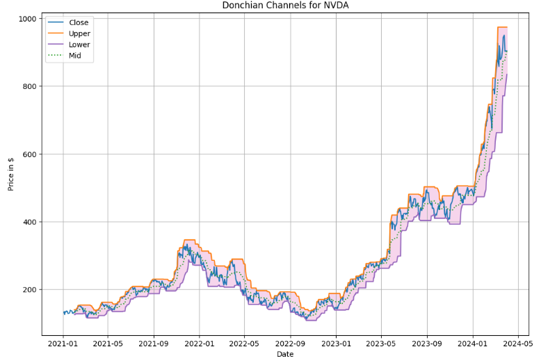

Comparing Cumulative Returns for Mid Donchian Cross-Over Strategy vs Buy-and-Hold default

midDon = midDonCrossOver(data.copy(), 20, shorts=False)

plt.figure(figsize=(12, 4))
plt.plot(midDon["strat_cum_returns"] * 100, label="Mid Don X-Over")
plt.plot(midDon["cum_returns"] * 100, label="Buy and Hold")
plt.title("Cumulative Returns for Mid Donchian Cross-Over Strategy")
plt.xlabel("Date")
plt.ylabel("Returns (%)")
plt.xticks(rotation=45)
plt.legend()
plt.grid()
plt.show()

stats = pd.DataFrame(getStratStats(midDon["log_returns"]), 
                     index=["Buy and Hold"])
stats = pd.concat([stats,
                   pd.DataFrame(getStratStats(midDon["strat_log_returns"]),
                               index=["MidDon X-Over"])])
stats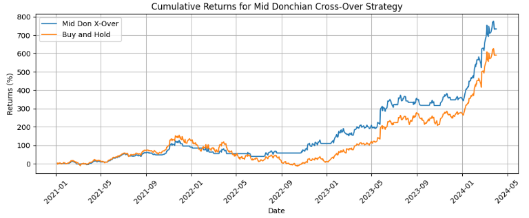

Cumulative Returns of NVDA for Mid Donchian Cross-Over Strategy vs Buy-and-Hold default

NVDA Risk/Return Summary: Mid Donchian Cross-Over Strategy vs Buy-and-Hold default.

Conclusions

In this study, we have performed the algo-trading technical analysis of NVDA using Donchian Channels (DC).
Results have shown that DC can provide valuable insights into NVDA stock dynamics and offer potential opportunities for profit and exit strategies.
It appears that NVDA Mid Donchian Cross-Over (Strategy 1) has outperformed the Buy-and-Hold default in terms of Cumulative Returns and popular Risk/Return KPIs for our selected timeframe.

Explore More

References

Embed Socials

Algo-Trading NVIDIA with Donchian Channels

Conclusions

Explore More

References

Embed Socials

Contacts