Building A Simple Breakout Trading System Using Python

Whether you are a beginner or an experienced trader, having a well-designed trading system can be an essential part of your investment strategy. A trading system is a set of rules that you follow to determine when to buy and sell, based on objective criteria rather than subjective judgment.

There are many different approaches to building a trading system, and the specific rules you choose will depend on your investment goals, risk tolerance, and other factors. In this project, I will build a trading system based on the Donchian Channel indicator.

The Donchian Channel is a popular trend-following indicator that can be a useful tool for traders looking to identify potential entry and exit points in the market. Developed by Richard Donchian, the Donchian Channel consists of a midline and two outer bands that are plotted a certain number of standard deviations above and below the midline.

You can use the midline as a trend filter, only taking long positions when prices are above the midline and short positions when prices are below the midline. The outer bands can be used as entry and exit points, with traders buying when prices touch the upper band and selling when they touch the lower band.

How to Calculate the Donchian Channel.

The Donchian Channel consists of an upper and lower bound which are calculated by taking the highest high and lowest low over the previous N periods. The midline is the average of the upper and lower bounds.

Here is the method to calculate the Donchian Channel using Python.

!pip install yfinance

import pandas as pd
import numpy as np
import matplotlib.pyplot as plt
import yfinance as yf

def calcDonchianChannels(data: pd.DataFrame, period: int):
  data["upperDon"] = data["High"].rolling(period).max()
  data["lowerDon"] = data["Low"].rolling(period).min()
  data["midDon"] = (data["upperDon"] + data["lowerDon"]) / 2
  return data

Historical data of ‘Amazon’ from 2018 to 2022 will be used to back test this trading strategy.

ticker = "AMZN"
yfObj = yf.Ticker(ticker)
data = yfObj.history(start="2018-01-01", end="2022-12-31").drop(
    ["Volume", "Stock Splits"], axis=1)
data = calcDonchianChannels(data, 20)
data.tail()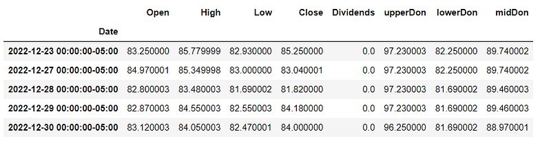

Let’s create a visualization of the Donchian Channel.

colors = plt.rcParams["axes.prop_cycle"].by_key()["color"]

plt.figure(figsize=(12, 8))
plt.plot(data["Close"], label="Close")
plt.plot(data["upperDon"], label="Upper", c=colors[1])
plt.plot(data["lowerDon"], label="Lower", c=colors[4])
plt.plot(data["midDon"], label="Mid", c=colors[2], linestyle=":")
plt.fill_between(data.index, data["upperDon"], data["lowerDon"], alpha=0.3,
                 color=colors[6])

plt.xlabel("Date")
plt.ylabel("Price in $")
plt.title(f"Donchian Channels for {ticker}")
plt.legend()
plt.show()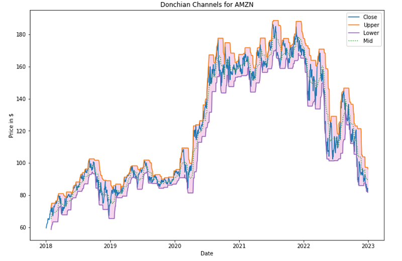

There are many variations of the Donchian Channel trading system, and you may want to experiment with different rules to see what works best for you. For example, you could use the outer bands as areas of support and resistance, or only take trades when the price breaks through the upper or lower band.

Now, we will dive in straight to the first variation which is Donchian Middle Value Cross-Over.

Strategy 1: Donchian Middle Value Cross-Over

This strategy will enter a position when the price closes above the midline value and will go short when the price drops below. The idea is to get those trends in the data when the close gets closer to the highs and vice versa.

def midDonCrossOver(data: pd.DataFrame, period: int=20, shorts: bool=True):
  data = calcDonchianChannels(data, period)

  data["position"] = np.nan
  data["position"] = np.where(data["Close"]>data["midDon"], 1, 
                              data["position"])
  if shorts:
    data["position"] = np.where(data["Close"]<data["midDon"], -1, 
                                data["position"])
  else:
    data["position"] = np.where(data["Close"]<data["midDon"], 0, 
                                data["position"])
  data["position"] = data["position"].ffill().fillna(0)

  return calcReturns(data)

Here are a few helper functions to give us returns and summary stats of the trading strategy. The summary will be used to compare the return of each strategy.

def calcReturns(df):
  df['returns'] = df['Close'] / df['Close'].shift(1)
  df['log_returns'] = np.log(df['returns'])
  df['strat_returns'] = df['position'].shift(1) * df['returns']
  df['strat_log_returns'] = df['position'].shift(1) * \
      df['log_returns']
  df['cum_returns'] = np.exp(df['log_returns'].cumsum()) - 1
  df['strat_cum_returns'] = np.exp(
      df['strat_log_returns'].cumsum()) - 1
  df['peak'] = df['cum_returns'].cummax()
  df['strat_peak'] = df['strat_cum_returns'].cummax()
  return df

def getStratStats(log_returns: pd.Series,
  risk_free_rate: float = 0.02):
  stats = {}  # Total Returns
  stats['tot_returns'] = np.exp(log_returns.sum()) - 1  
  
  # Mean Annual Returns
  stats['annual_returns'] = np.exp(log_returns.mean() * 252) - 1  
  
  # Annual Volatility
  stats['annual_volatility'] = log_returns.std() * np.sqrt(252)
  
  # Sortino Ratio
  annualized_downside = log_returns.loc[log_returns<0].std() * \
    np.sqrt(252)
  stats['sortino_ratio'] = (stats['annual_returns'] - \
    risk_free_rate) / annualized_downside  
  
  # Sharpe Ratio
  stats['sharpe_ratio'] = (stats['annual_returns'] - \
    risk_free_rate) / stats['annual_volatility']  
  
  # Max Drawdown
  cum_returns = log_returns.cumsum() - 1
  peak = cum_returns.cummax()
  drawdown = peak - cum_returns
  max_idx = drawdown.argmax()
  stats['max_drawdown'] = 1 - np.exp(cum_returns[max_idx]) \
    / np.exp(peak[max_idx])
  
  # Max Drawdown Duration
  strat_dd = drawdown[drawdown==0]
  strat_dd_diff = strat_dd.index[1:] - strat_dd.index[:-1]
  strat_dd_days = strat_dd_diff.map(lambda x: x.days).values
  strat_dd_days = np.hstack([strat_dd_days,
    (drawdown.index[-1] - strat_dd.index[-1]).days])
  stats['max_drawdown_duration'] = strat_dd_days.max()
  return {k: np.round(v, 4) if type(v) == np.float_ else v
          for k, v in stats.items()}

Let’s test this on our historical data of Amazon stock.

midDon = midDonCrossOver(data.copy(), 20, shorts=False)

plt.figure(figsize=(12, 4))
plt.plot(midDon["strat_cum_returns"] * 100, label="Mid Don X-Over")
plt.plot(midDon["cum_returns"] * 100, label="Buy and Hold")
plt.title("Cumulative Returns for Mid Donchian Cross-Over Strategy")
plt.xlabel("Date")
plt.ylabel("Returns (%)")
plt.xticks(rotation=45)
plt.legend()

plt.show()

stats = pd.DataFrame(getStratStats(midDon["log_returns"]), 
                     index=["Buy and Hold"])
stats = pd.concat([stats,
                   pd.DataFrame(getStratStats(midDon["strat_log_returns"]),
                               index=["MidDon X-Over"])])
stats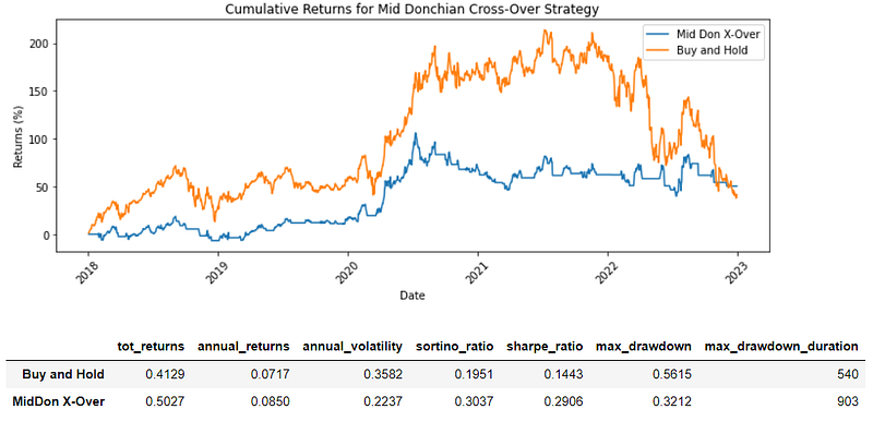

We can observe clearly that Donchian Middle Value Cross-Over strategy has a better total return compared to the “Buy-and-Hold” strategy.

Strategy 2: Donchian Channel Breakout

When prices breakout above the upper band of the Donchian Channel, it is often seen as a bullish signal, indicating that the market is experiencing upward momentum and that prices may continue to rise. Conversely, when prices breakout below the lower band of the Donchian Channel, it is often seen as a bearish signal, indicating that the market is experiencing downward momentum and that prices may continue to fall.

The basic idea of this strategy is to go long when the price breaks through the upper channel and short or exit the trade if it breaks below the lower channel. Because we’re looking at high prices, we’ll define a breakout as a close that’s greater than yesterday’s Donchian bound.

def donChannelBreakout(data, period=20, shorts=True):
  data = calcDonchianChannels(data, period)
  
  data["position"] = np.nan
  data["position"] = np.where(data["Close"]>data["upperDon"].shift(1), 1, 
                              data["position"])
  if shorts:
    data["position"] = np.where(
      data["Close"]<data["lowerDon"].shift(1), -1, data["position"])
  else:
    data["position"] = np.where(
      data["Close"]<data["lowerDon"].shift(1), 0, data["position"])
      
  data["position"] = data["position"].ffill().fillna(0)
  
  return calcReturns(data)

We can test it on our data just like we did above.

breakout = donChannelBreakout(data.copy(), 20, shorts=False)

plt.figure(figsize=(12, 4))
plt.plot(breakout["strat_cum_returns"] * 100, label="Donchian Breakout")
plt.plot(breakout["cum_returns"] * 100, label="Buy and Hold")
plt.title("Cumulative Returns for Donchian Breakout Strategy")
plt.xlabel("Date")
plt.ylabel("Returns (%)")
plt.xticks(rotation=45)
plt.legend()

plt.show()

stats = pd.concat([stats,
                   pd.DataFrame(getStratStats(breakout["strat_log_returns"]),
                               index=["Donchian Breakout"])])
stats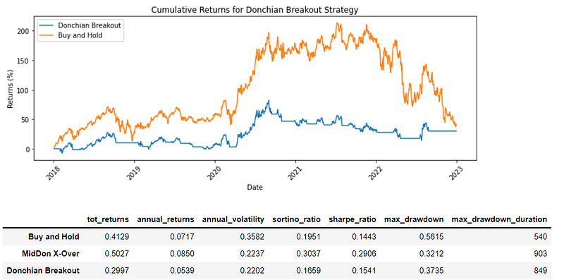

Conclusion

Based on the results, it is clearly that Donchian Middle Value Cross-Over strategy gives the highest total return after ‘buy-and-hold’ strategy if the trades were made from 2018 to 2022 for Amazon stock.

In my opinion, the return from both Donchian Channel strategies can be maximised by having a good risk management.

It is important to remember that no single trading system is right for everyone, and the Donchian Channel may not be appropriate for all investors or market conditions. As with any trading strategy, it is essential to carefully consider your investment objectives and risk tolerance before using the Donchian Channel or any other trading system.