Business Forecasting with Facebook’s “Prophet”

Virtually every business decision and process is based on a forecast. A company uses its past sales data to forecast what its sales volume will be for the next 12 months. The forecasts help the company to allocate what resources (such as employees) might be required to meet the demand.

Business forecasting can be very challenging. First, the time series itself may require specific domain knowledge about the business such as any particular spikes in the past years. Second, there exists a huge list of quantitative forecasting methods that may become additional burdens for data analysts. Third, the forecasting process should be fast and interpretable.

In this article I will demonstrate the “Prophet” module, open-sourced by Facebook.com, to produce forecasts for planning and goal setting. It is available in both R and Python on Github. “Prophet” is easy to use.

I have also written tutorial posts on NeuralProphet, a successor to Facebook Prophet. You are invited to read

• NeuralProphet (I) — Trend + Seasonality + Holidays and
• NeuralProphet (II) — AR + Lagged and Future Regressors.

Great. Let’s start with the fundamentals.

Behind the Scene — the Generalized Additive Model (GAM)

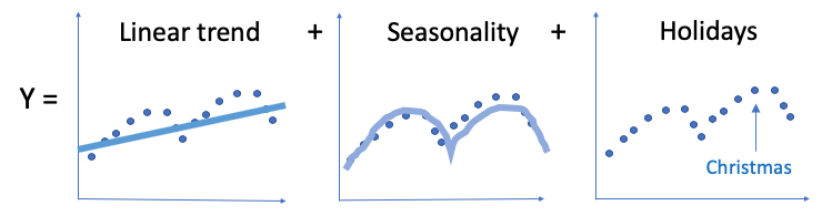
A business time series can be characterized by a long-term linear trend, a yearly seasonal effect, and any holiday effect like the following:

GAM is an intuitive selection. In the article “Explain Your Model with Microsoft’s InterpretML” I explained GAM. It was originally invented by Trevor Hastie and Robert Tibshirani in 1986. Although GAM does not receive sufficient popularity yet as a random forest or gradient boosting in the data science community, it is certainly a powerful and yet simple technique. The idea of GAM is intuitive:

• Relationships between the individual predictors and the dependent variable follow smooth patterns that can be linear or nonlinear. Figure (A) illustrates the relationship between x1 and y can be nonlinear.
• Additive: these smooth relationships can be estimated simultaneously and then added up.

A business time series can be specified by GAM with the following components:

y(t) = g(t) + s(t) + h(t) + ε(t)

• Trend: g(t),
• Seasonality: s(t) for weekly and yearly seasonality,
• Holiday Effects: h(t) for the effects of holidays that occur on potentially irregular schedules over one or more days,

and ε(t) is for any idiosyncratic changes which are not accommodated by the model. The predictor is t or time.

What Kind of Time Series that the Prophet Is Good at?

So if a time series can be formulated by the time such as year, season, month, or week, the “Prophet” will be a good choice. How about other types of time series? In the second half of the article, I will show you a macroeconomic time series to see what the model picks up.

Time Series Articles

If you are looking for a comprehensive survey on time series forecasting and anomaly detection, below is a list that you may find helpful:

• Part 1: “Anomaly Detection for Time Series“
• Part 2: “Detecting the Change Points in a Time Series”
• Part 3: “Algorithmic Trading with Technical Indicators in R”
• Part 4: “Kalman Filter Explained!”
• Part 5: “Business Forecasting with Facebook’s “Prophet”
• Part 6: “Time Series with Zillow’s Luminaire — Part I Data Exploration”
• Part 7: “Time Series with Zillow’s Luminaire — Part II Optimal Specifications”
• Part 8: “Time Series with Zillow’s Luminaire — Part III Modeling”
• Part 9: “A Technical Guide on RNN/LSTM/GRU for Stock Price Prediction”

(A) “Prophet” Is Easy to Use

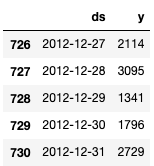
I am going to model the Bike Share Daily data from Kaggle here or here. Bike-sharing systems are the new version of traditional bike rentals. A user can easily rent a bike from a particular location and return to another location. The bike-sharing daily count is highly correlated to weather conditions and seasonality (day of week and season). “Prophet” requires two columns with the names “ds” and “y”. You can download the notebook via this link.

Do a pip install prophet or visit the Prophet homepage for the installation guide. A reader encountered an installation issue. I helped and documented at the end of the article in case other readers encounter similar issues.

(A.1) The Default Model

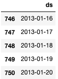
Below I adopt the default setting to build the default model. I also generate 20 data points for the future period. I then apply the model to forecast them. Let me break down the steps:

• Line 2–3: Line 2 declares a default model ‘bike_model_0’. The model training is in Line 3.
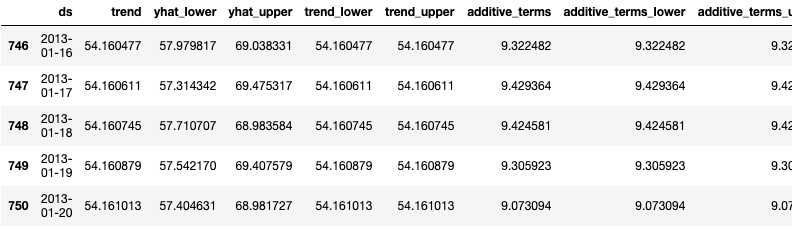
• Line 6: The make_future_dataframe() generates 20 points according to Trend: g(t), Seasonality: s(t) for weekly and yearly seasonality, and Holiday Effects: h(t).
• Line 10: It takes the generated data to produce 20 forecasts, i.e., y(t).

(A.2) Automatic Change Point Detection in Prophet

The trend component does not need to be a single straight line. It can be a connected piecewise line with many change points. Do you know change point detection is an important topic in time series? Take a look at “Detecting the Change Points in a Time Series” and then you will get good answers.

The “Prophet” allows a large number of (up to 29) potential change points. The algorithm uses L1 regularization to keep the change points as few as possible. If this is the first time you hear L1 regularization, it is absolutely fine. In short, it is a machine learning technique to prevent overfitting. What’s the problem if you overfit a time series? It works perfectly well with the current training data but has very little predictability for future data. See “My Lecture Notes on Random Forecast, Gradient Boosting, Regularization, and H2o.ai” for more detail.

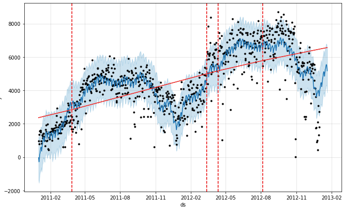
The model identified four change points (shown by the four dashed lines). If you have the domain knowledge that the trend changed on certain days, you can also specify the locations of the trend changes, click here.

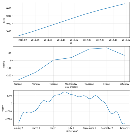
The above result is very satisfactory. The decomposition shows the “trend”, the “weekly” pattern, and the “monthly” pattern.

(A.3) Fit the Trend Flexibly

We may overfit the trend changes (too much flexibility) or under-fit (not enough flexibility). It can be controlled by changepoint_prior_scale. By default, this parameter is set to 0.05. Increasing it will make the trend more flexible. Below I change it to 0.1. The results may look similar to the default model. It means the default model has already done a good job. Later in the second example, you will see this parameter can impact quite a lot.

(A.4) Diagnostics

How do we evaluate the predictability of a time series model? An intuitive way is to “backtest” the model with past data. If we select a cutoff point in the history, fit the model using data only up to that cutoff point, and provide forecasts after that cutoff point. We can then compare the forecasted values to the actual values. We can select multiple cutoff points in the history to provide the model diagnostics.

Below is a code snippet for model diagnostics. The size of the training data is defined by the parameter initial for 100 days. The parameter horizon means to the forecasting horizon. The 365 days means we want to provide the forecasts for 365 days after the cutoff date. Finally, we will select multiple cutoff points to build multiple models. The parameter period specifies the period between models. It says the next cutoff point is 180 days after the previous cutoff point.

# Diagnostics 0
from prophet.diagnostics import cross_validation
bike_0_cv = cross_validation(bike_model_0, 
                         initial='100 days', 
                         period='180 days', 
                         horizon = '365 days')
bike_0_cv.head()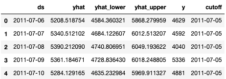

The performance_metrics utility produces some useful statistics (yhat, yhat_lower, and yhat_upper compared to y): mean squared error (MSE), root mean squared error (RMSE), mean absolute error (MAE), mean absolute percent error (MAPE), and coverage of the yhat_lower and yhat_upper estimates.

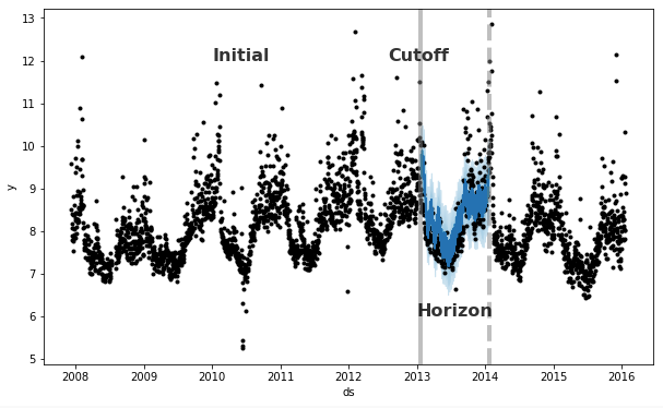
The cross_validation function automatically computes a range of historical cutoffs, as shown in the graph below:

• The forecast horizon (horizon)
• The initial training period (initial): optional
• The spacing between cutoff dates (period)

By default, the initial training period is set to three times the horizon, and cutoffs are made every half a horizon.

We can compare the performances of the two models:

# Performance 0
from prophet.diagnostics import performance_metrics
bike_0_p = performance_metrics(bike_0_cv)
bike_0_p.head()

# Performance 2
bike_2_p = performance_metrics(bike_2_cv)
bike_2_p.head()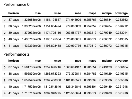

(B) Does the “Prophet” Model Fit Well for a Macroeconomic Time Series?

We know the “Prophet” module models a time series with the “trend”, “seasonality” (weekly or yearly), and “holidays”. Can the module model the PMI well?

In the article “Plot the U.S. Economic Leading Indicator PMI with Plotly”, we know the U.S. Purchasing Managers Index (PMI) for manufacturing is “one of the hottest economic indicators” as described by Bernard Baumohl in his best-selling book The Secrets of Economic Indicators. The PMI has demonstrated a solid track record of anticipating turning points in the business cycle and being way ahead of the curve in detecting a buildup of inflation pressures. The plot below shows how the PMIs correspond with recessions (in orange color).

We obtain the same PMI data for modeling.

import pandas as pd
from prophet import Prophet
from prophet.plot import plot_plotly

pmi = pd.read_csv('ISM-MAN_PMI.csv')
pmi = pmi[pmi.Date>='1981-01-01']
pmi

ts = pd.DataFrame()
ts['ds'] = pd.to_datetime(pmi["Date"])
ts['y']  = pmi['PMI']

from prophet.plot import add_changepoints_to_plot
model_0 = Prophet(#n_changepoints=20, 
                  yearly_seasonality=True, 
                  changepoint_prior_scale=0.4
                   )

# Fitting with default parameters
model_0.fit(ts)
future= model_0.make_future_dataframe(periods=20, freq='M')
model_0_forecast=model_0.predict(future)
fig = model_0.plot(model_0_forecast)
a = add_changepoints_to_plot(fig.gca(), model_0, model_0_forecast)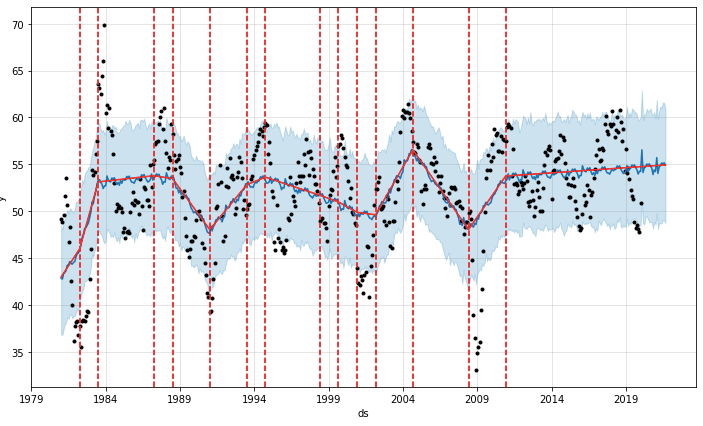

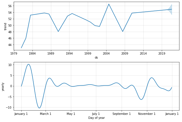
The “trend” component is segmented, as shown in the red solid line above and the blue line below. The “seasonality” component shows the month of February is typically the lowest. How does the model capture the multi-year changes in a macroeconomic time series? It assigns to the changes in the “trend” component.

Installation Error: One reader encountered an error in pip install fbprophet. The reader runs on a virtual environment of Anaconda 3.8 on his Mac. I helped and found his Mac should install Xcode by running xcode-select --install, see this post, which seems a common technical issue. I am certainly not an expert in Mac. Here I just document this technical issue in case other readers also encounter this challenge.

Readers are recommended to purchase books by Chris Kuo:

• The explainable AI: https://a.co/d/cNL8Hu4
• Transfer learning for image classification: https://a.co/d/hLdCkMH
• Modern time series anomaly detection: https://a.co/d/ieIbAxM
• Handbook of Anomaly Detection: https://a.co/d/5sKS8bI