Detecting the Change Points in a Time Series

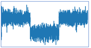
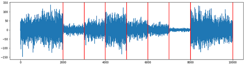
Suppose you wear an iWatch to monitor your heart rate. You run for a quarter mile, walk for ten minutes, then run for another quarter mile. The heart rate data will look like the time series in Figure 1. It shows a cluster of high heart rates, then a cluster of low heart rates, then back to high rates. The abrupt changes in the time series inform us the source object has major activity changes. Similarly, imagine a patient in an Intensive Care Unit (ICU), and the nurses monitor his heart rate. It is critical to detect any changes in the heart rate and alert the doctor to respond quickly. We need to detect them accurately and timely and send out alarms. Change point detection (CPD) is important. In medical condition monitoring, we need to monitor the health condition of a patient; in speech recognition, we detect the changes in the voice frequencies; in weather detection, we monitor the temperature changes to signal the citizens.

(A) Where Does CPD Fit in a Typical Data Science Process?

A typical data science process can be described by the flowchart in Figure (A): Data Preparation → Model Specification → Modeling → Forecasting. The data preparation step includes exploratory data analysis, data cleaning, and missing data imputation. Change point detection is an important task in the data preparation step.

With prepared data, the model specification step searches for the best model specifications to do modeling. This step collects the basic information about the time series. For example, What is the frequency of the time series? Where are the change points? Do we need a logarithmic transformation? Should some of the data points be truncated? Do you need flags for the holidays? Should you apply Fourier transformation, and with what frequency? These tasks are frequently performed by an experienced data scientist. The good news is that they are incorporated into many modules for automation.

The modeling step models the data for an appropriate model. These models include a structural model such as ARIMA or Decomposition, as well as a moving average or a Kalman Filter model. The forecasting considers how users need the forecasts such as real-time predictions, or streaming data anomaly detection.

(B) Why Read this article?

In this article, I will introduce several CPD algorithms. After reading this article you will understand why it is important to develop different algorithms for real-time (online) or batch (offline) applications. You will also learn the reasons why CPD has been employed by many forecasting Python tools such as the Luminaire by Zillow, or the Prophet/Kats by Facebook.

(C) Real-time (Online) and Batch (Offline)

With a time series long enough, you can spot the change points easily. Some algorithms use all the past data to detect changes. However, there are real-time use cases where you cannot afford to collect data over a long period to determine the change points. For example, suppose you fly a drone that streams its positions every second to the home device. You cannot just wait and collect data over ten minutes to detect any changes retrospectively. With the emergence of real-time streaming data such as IoT or online streaming, online methods can be implemented on a hardware device (see [2]). Because of the real-time and non-real-time use cases, both the real-time (or called online) and the batch (or called offline) algorithms have been developed to provide efficiency.

The offline algorithm uses the entire time series (or at least the time series of a longer period) to detect the changes. In contrast, online algorithms can detect the change points “on the fly”. I will show you the Ruptures Python module for offline applications, and the changefinder module for online applications.

(D) Generate Two Time Series

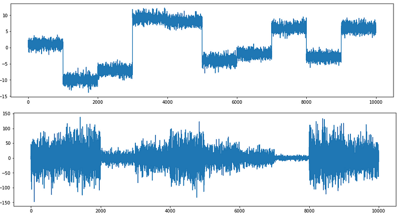
I generate two-time series to test the algorithms that I am going to introduce. The change points in the first time series are easier to detect, and those of the second one is harder to detect. The notebook is available via this Github link.

• The first time series “ts1”: Has ten data segments with constant variance.
• The second time series “ts2”: has ten data segments but with varying variances.

(E) Offline — The Ruptures Module

In time series modeling we try to find the underlying pattern such as a regression line so we can forecast the future. But the regression line will not be straight if there are change points. So an intuitive algorithm is to build segmented regression lines where the kinked points are the change points. This method is called Pruned Exact Linear Time (PELT) [3], [4].

This regression-based algorithm can be explained by the two graphs (A) and (B) below. The time series (shown in blue) has one change point and two segments. The horizontal orange line in the left graph (A) is the regression line. The distance from each point (shown as a white circle) to the regression line is represented by the vertical orange line. The regression line is determined by minimizing the sum of the distances to all the data points.

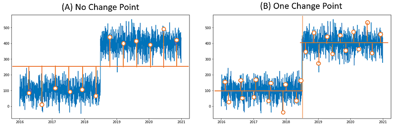
The regression line in (B) is cut into two regression lines at the change point. The sum of the distances in (B) is much smaller than that in (A). By sliding the cut point from left to right of the time series, the algorithm can find the appropriate change point for the time series that minimizes the sum of the distances or errors. The equation below is the algorithm to search for the number of change points and the locations of change points. C(.) is the distance or the cost function. We also need to control for not creating too many line segments thus overfitting the time series. So the term b (beta) is the number of segments as a penalty term to prevent the search from yielding too many segments.

This algorithm is coded in the Python module “ruptures”. Let’s see how it works. Install it with pip install ruptures.

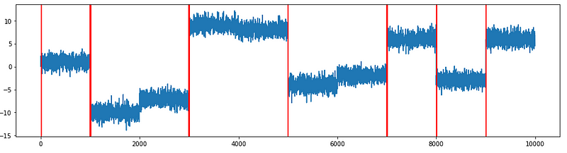
Example E.1 — constant variance

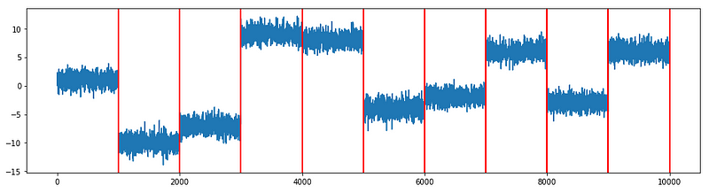
This is nice. It has detected all the ten change points that we have generated. Let’s see if it is still effective when the variance varies over time.

Example E.2 —varying variance

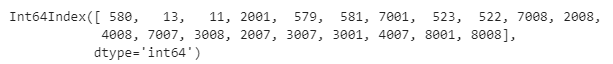
The PELT algorithm spots the changing points at [2000, 3000, 3990, 5005, 5995, 6995, 8000, 10000] as shown below. We know two change points [1000, 9000] are supposed to be there. But because the data before and after those points are too similar, PELT does not spot the difference.

The algorithm needs a long runtime to find the change points in Example 1.1 and especially Example 1.2. This may not meet the requirement for real-time streaming data. Therefore the following Python module “changefinder” is designed for real-time applications.

(F) On-line (real-time) — The changefinder Module

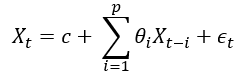
A time series can be characterized by an autoregressive (AR) moving average process. An AR model says the next data point is a weighted moving average of the past data points with a random noise like the following equation, in which θi are the weights of the past p data points.

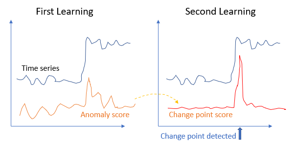
If there is a change point, it is expected that the AR processes before and after the change point will be different. With this intuition, Yamanishi & Takeuchi [5] proposed the Sequentially Discounting AutoRegressive (SDAR) learning algorithm. The SDAR method has two learning phases. In the first learning phase, it produces an intermediate score called the anomaly score. In the second learning phase, it produces the change-point score that can detect a change point. I outline the algorithm as the following:

• [1st AR model] Read in a chunk of data t = 1, …, N, then build an AR (auto-regressive) model. It then produces an “anomaly score” which is the difference between the AR predicted value for Xt and the actual data Xt. Notice in this step only N data points are taken. Since it does not use the entire history, it is set for an online stream of data.
• [1st Smoothing] The above anomaly score will be very volatile and produce false signals. The algorithm generates the moving average Yt for the anomaly score to smooth out the outliers.
• [2nd AR model] Build an AR model for Yt and produce another “anomaly score” based on the newly built AR model and Yt.
• [2nd Smoothing] Similarly, the new anomaly score tends to be volatile. The algorithm generates the moving average to smooth out. The final product is a score called the change-point score, as shown in the illustration below.

This algorithm does not need the entire time series to detect change points so it substantially reduces the computation time. In the following Example 2.1 and Example 2.2 I will test the algorithm on the two simulated time series data generated in Section (0). The first one (ts1) is a time series with constant variance, and the second one (ts2), has a varying variance.

Example F.1 —constant variance

We are interested in the change-point score in the changefinder module that indicates if a time series departs abruptly from its norm. The code below applies the model to the first time series (ts1). The code has three parameters:

• r: the discount rate (0 to 1). If you set a high discount rate, the past time series decreases quickly, meaning you do not want to learn from the past. Setting it at 0.01 is just fine. It is not very sensitive so it does not matter if it is set at 0.01 or 0.05. Experiment with it.
• order: the AR model order
• smooth: the widow size of recent N data to compute the moving average for smoothing.

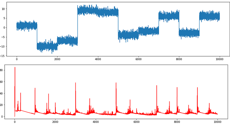
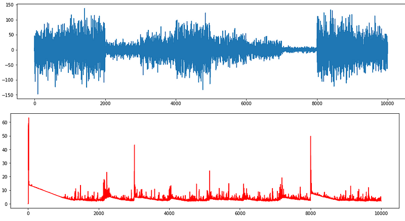
The red time series is the change-point score. Those large change-point scores are the locations where changes happen. Here I print out the locations of the top 20 (you can take more).

I plot these detected change points on the time series to see how well the change points were detected. In general, the algorithm does a decent job of finding those change points. The method missed the change points at 2000, 4000, and 6000. This is because the data frequency before and after those points are too similar to qualify for a difference. While running the code, you may find the computational time is much less than the PELT method of the ruptures module.

Example F.2 — varying variance

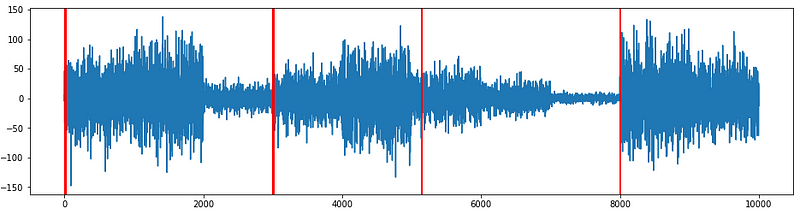
Change points in a time series with varying variance are hard to find. As shown below, Time series ts2 seems to have three to four clusters, not ten clusters as we designed. Let’s test the performance of the algorithm. The red time series is the change-point score. It detects several change points.

I plot the change points on the time series ts2. Considering the complexity of the time series, the result is quite reasonable.

(G) Conclusion

I hope this article gives you a better understanding of this topic. If you like to have a comprehensive review, the following sequence will help:

• Part 1: “Anomaly Detection for Time Series“
• Part 2: “Detecting the Change Points in a Time Series”
• Part 3: “Algorithmic Trading with Technical Indicators in R”
• Part 4: “Kalman Filter Explained!”
• Part 5: “Business Forecasting with Facebook’s “Prophet”
• Part 6: “Time Series with Zillow’s Luminaire — Part I Data Exploration”
• Part 7: “Time Series with Zillow’s Luminaire — Part II Optimal Specifications”
• Part 8: “Time Series with Zillow’s Luminaire — Part III Modeling”
• Part 9: “A Technical Guide on RNN/LSTM/GRU for Stock Price Prediction”

[1] C. Truong, L. Oudre, N. Vayatis. A selective review of offline change point detection methods. Signal Processing, 167:107299, 2020. [journal] [pdf]

[2] Takuma Iwata , Kohei Nakamura, Yuta Tokusashi, and Hiroki Matsutani. Accelerating Online Change-Point Detection Algorithm using 10GbE FPGA NIC. [pdf]

[3] Killick Rebecca, Fearnhead P, Eckley Idris A(2012). Optimal detection of change points with a linear computational cost. JASA, 107, 1590–1598 (arxiv_link)

[4] Gachomo Dorcas Wambui, Gichuhi Anthony Waititu, Jomo Kenyatta (2015). The Power of the Pruned Exact Linear Time(PELT) Test in Multiple Changepoint Detection American Journal of Theoretical and Applied Statistics Volume 4, Issue 6, November 2015, Pages: 581–586 (arxiv_link)

[5] Yamanishi, K., & Takeuchi, J. I. (2002). A unifying framework for detecting outliers and change points from non-stationary time series data. 676–681. Paper presented at KDD — 2002 Proceedings of the Eight ACM SIGKDD International Conference on Knowledge Discovery and Data Mining, Edmonton, Alta, Canada. https://doi.org/10.1145/775047.775148

[6] Militino, A.F.; Moradi, M.; Ugarte, M.D. On the Performances of Trend and Change-Point Detection Methods for Remote Sensing Data. Remote Sens. 2020, 12, 1008. https://doi.org/10.3390/rs12061008

Time Series Articles

If you are interested in a comprehensive survey on time series forecasting and anomaly detection, below is a list that you may find helpful:

• Part 1: “Anomaly Detection for Time Series“
• Part 2: “Detecting the Change Points in a Time Series”
• Part 3: “Algorithmic Trading with Technical Indicators in R”
• Part 4: “Kalman Filter Explained!”
• Part 5: “Business Forecasting with Facebook’s “Prophet”
• Part 6: “Time Series with Zillow’s Luminaire — Part I Data Exploration”
• Part 7: “Time Series with Zillow’s Luminaire — Part II Optimal Specifications”
• Part 8: “Time Series with Zillow’s Luminaire — Part III Modeling”
• Part 9: “A Technical Guide on RNN/LSTM/GRU for Stock Price Prediction”

Readers are recommended to purchase books by Chris Kuo:

• The explainable AI: https://a.co/d/cNL8Hu4
• Transfer learning for image classification: https://a.co/d/hLdCkMH
• Modern time series anomaly detection: https://a.co/d/ieIbAxM
• Handbook of Anomaly Detection: https://a.co/d/5sKS8bI