Kalman Filter Explained!

The local beach is not far from where I live, so sometimes I go there to enjoy my solitude. Today I was meditating on tomorrow’s lecture on Kalman Filter. “It could be a challenging concept for some students”, I said to myself. I sat on a large rock, felt the gentle breeze, and soaked in the warm sunset. I watched the seagulls flying over the majestic sunset, casting fuzzy reflections on the sparkling ocean. Suddenly I have an indescribable joyful moment — the line of the flying seagull in the sky and the fuzzy reflections on the ocean is a beautiful analogy for the Kalman Filter. I shouted to the seagulls “A-ha”, and they echoed me with “A-ha-A-ha-A-ha”.

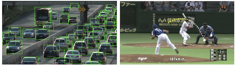
If this is the first time you've heard of the Kalman Filter, you may not know that numerous devices in our lives have relied on it. The Kalman Filter estimates the trajectory of a moving object. Your iPhone or Android phone has a map app that estimates the location of the phone and driving distance. Cars, fleet trucks, ships, aircraft, or drones have the GPS (Global Positioning System) to track movement with more accuracy. A famous early use was the Apollo navigation computer that took Neil Armstrong to the moon and, most importantly, brought him back. The Kalman Filter also is widely applied in time series anomaly detection. With the advent of computer vision to detect objects in motions such as cars or baseball curves, the Kalman Filter model will become even more significant.

In this article I will start with the basic concept, then the algorithm, and the Python code. I will show you three cases. The first one is its application in stock price modeling, and the second and third ones explain its applications for a moving object. The Python notebook is available via this Github.

(A) Where Does the Kalman Filter Fit in a Typical Data Science Process?

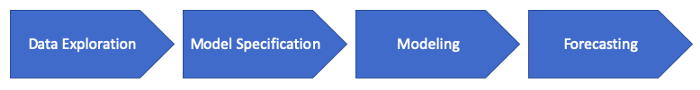
A typical data science process can be described by the flowchart in Figure (A): Data Preparation → Model Specification → Modeling → Forecasting. The data preparation step includes exploratory data analysis, data cleaning, and missing data imputation. The Kalman Filter is a modeling technique that fits in the modeling step. It is also incorporated in the Luminaire module, see Part 8: “Time Series with Zillow’s Luminaire — Part III Modeling”

(B) The Story of the Flying Seagull

Imagine you fixed your eyes on the sparkling reflections, shown as Yt at the beginning of the article. You know it comes from the flying line of the seagull in the sky Xt, but you cannot observe Xt at the same time. Meanwhile, the wavy ocean makes the projected Yt very noisy.

This story captures several salient properties of the Kalman Filter: (1) the location Xt of the flying seagull depends on the prior location at t-1. Xt is called the state at time t and is not observable. (2) The observable Yt comes from the unobservable Xt, with Gaussian noises. The Kalman Filter can recover the “true state” Xt, given a sequence of noisy Yt.

Let me introduce the model in its mathematical form. I will use the simplest form of the Kalman Filter that has one term Xt-1 and the error term. The location of the flying seagull at time t is Xt, which depends on the prior location Xt-1, multiplying the transition matrix At, plus a random Gaussian noise qt.

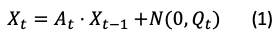
The transition matrix tells us how the location changes from the previous state to the current state. The transition matrix evolves and is not a constant. In this simple one-term equation the transition matrix is just a numerical value. Let’s still accept the conventional notation as a matrix. Later in the article, I will introduce more terms in the equation, then you will see it is a matrix. The error term qt has its covariance matrix Qt. A covariance matrix is a square matrix giving the covariance between each pair of elements of a given random vector. In this simple one-term equation, the random vector has only one element and the covariance is just a single value.

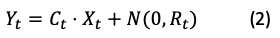
Now let me introduce the second equation. The location of the reflection is Yt. It is the state Xt, multiplying the observation matrix Ct, plus a white noise rt. The observation matrix tells us the next observation (or called measurement) we should expect given the predicted state Xt. The covariance matrix of the error rt is Rt. Again, in this single measure case, the covariance is a single value.

(C) How Does the Kalman Filter Work with GPS?

GPS is a system of 30+ navigation satellites circling Earth. They constantly send out signals. A GPS receiver in your phone gets these signals. The receiver calculates its distance from four or more GPS satellites to figure out your location.

But the signals traveling through the sky to your receiver are not without errors. The fuzzy blue line in the following image is likely what your GPS receiver gets, the smooth orange line is what you see in your app. The Kalman Filter algorithm “filters out” the rough blue line to get the orange line.

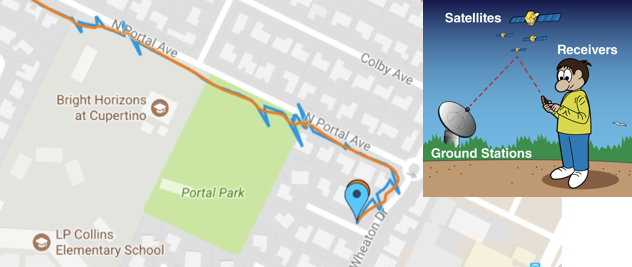
How do the two equations apply to this story? In Equation (1), the location of the car is Xt, which transits from the prior location Xt-1 by the transition matrix At, plus some white errors. The GPS has a measurement error too. In Equation (2), Yt is the observed location in my GPS receiver. It is projected from the true location Xt through the observational matrix Ct, plus the satellite-GPS measurement errors qt. The GPS receiver in my phone applies the Kalman Filter to get Xt from the observable Yt.

(D) Why Use the Word “Filter”?

A noisy time series is like a time series with many rough edges. The Kalman Filter estimates the underlying states. It “filters” out the rough edges to reveal relatively smooth patterns. (There is nothing to do with your coffee filter, lol.) The filter is named for Rudolf (Rudy) E. Kálmán, who is one of the primary developers of its theory.

Notice that “smoothing” is different from the smoothing of moving average methods. The moving average methods take the past points, even errors, with differential weights to get a smoothed line. In contrast, the Kalman Filter recognizes some data points as noise. It finds the underlying Xt.

(E) The Key Properties of the Kalman Filter

Let me summarize some key properties here:

• A Kalman filter is called an optimal estimator. Optimal in what sense? The Kalman filter minimizes the mean square error of the estimated parameters. So it is the best-unbiased estimator.
• It is recursive so that Xt+1 can be calculated only with Xt. and does not require the presence of all past data points X0, X1, …, Xt. This is an important merit for real-time processing.
• The error terms in Equations (1) and (2) are both Gaussian distributions, so the error term in the predicted values also follows the Gaussian distribution.
• There is no need to provide labeled target data to “train” a model.

(F) How Does the Algorithm Work?

Let me break down the mathematical operations of the Kalman Filter into steps.

1. Initiate the state value X0. Since we do not know anything about it, we just provide any value for X0. You will see how the Kalman Filter converges to the true value. Get the initial values for the transition matrix A0, the operational matrix C0, and the covariance matrix of the error Wt and Vt.
2. Predict: The Kalman Filter estimates the current state Xt using the transition matrix At for time step t.
3. Update: The Kalman Filter obtains the new observation Yt as a new input. Then it estimates the covariance matrix Qt and Rt for time step t.
4. Repeat Steps (2) and (3) for the next time step. In each step, it only needs the statistics of the previous time t-1 but not the entire history.

(G) The Kalman Filter for the Stock Price Prediction

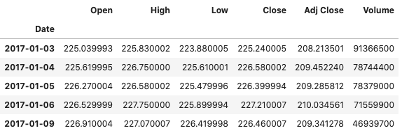
Stock price movement is widely modeled as a random walk. It means at each point in time the series merely takes a random step away from its last position, with steps that the mean value is zero. This is described in Equation (1) describes: Xt = At * Xt-1. when At = 1. This is also called random-walk-without-drift. (For your reference, if the mean step size is a nonzero value α, it is called random-walk-with-drift. It becomes Xt = At * Xt-1 + α.) Below let’s download the S&P 500 through the yfinance API.

It is straightforward to implement the Kalman Filter. Equation (1) only has one term Xt-1. So the transition matrix At only has one value [1.0]. It is 1.0 because of the random walk assumption. We also allow it to have small turbulence of 0.01, meaning the At can sometimes go above 1.0 and sometimes go below 1.0. It is denoted by transition_covariance=0.01. The observation matrix Ct also is 1.0.

How about the initial value X0? You can enter any value (assume we know nothing about the S&P 500). Later you’ll see how it quickly converges to the true value. The error terms qt and rt are Gaussian-distributed with a mean of 0 and variance of 1.0. So initial_state_covariance=1 and observation_covariance=1.

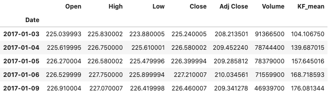
We store the Kalman Filter estimates in Column “KF_mean”. Do you see the first few estimates are far off from the target “Adj Close”? However, it converges to the target “Adj Close” after the first few observations, as shown in the plot below.

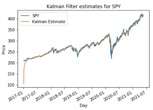
Do you notice we do not set up a training dataset to train the model? That’s correct. The Kalman Filter does not work that way. The purpose of training a model is to get the parameters At. The Kalman Filter gets a parameter value for each new time step t.

(H) The Kalman Filter for a Moving Object

(H) Method 1

A moving object such as a ball or a car is typically controlled by a force, so not only its position changes over time but also its velocity changes over time. Now the state vector Xt can have two elements: position and velocity, and both are unobservable. I include this Case 2.1 to show you how to set up the transition and the observation matrices when Xt is a vector.

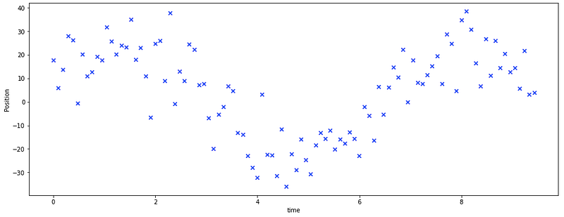
Let’s assume an object moves up and down over time, and the sensor detects it with a small error. I postulate a perfect sine wave with randomness for the movement over time. When the location is plotted over time, it looks like the following:

Now the state vector Xt has two elements “position” and “velocity”, i.e., Xt = [xt, vt]. According to physics, the new location is the previous location plus velocity multiplying time: xt = xt-1+ v⋅t. We assume velocity does not change, although there is small turbulence, so vt = vt-1. Equation (1) becomes the matrix form:

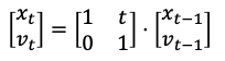
So the transition matrix At is [[1,t],[0,1]], where t = 1 in our case. We allow small turbulence for At, so the transition covariance transition_covariance builds in small turbulence.

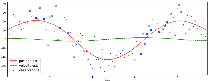
Let’s plot the observable Yt, and the Kalman Filter estimates for xt and vt. You will be amazed how the Kalman Filter restores the xt to a perfect sin wave if vt is assumed in the equation.

(H.2) Method 2

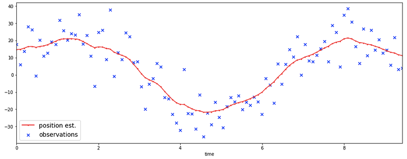
What if the transition matrix in Case 2.1 is set up as a single element? That means there is no velocity term in Xt. The Kalman Filter estimates for the positions. It does the job, but the zigzag estimates are far less perfect than a sin wave.

(I) Other Interesting Resources

This website simulates the Kalman Filter. Move your mouse around the screen. See how the Kalman Filter reduces the input noise and predicts your movement.

For the derivation of the predictions, I recommend the article “Understanding the Basis of the Kalman Filter via a Simple and Intuitive Derivation” published in IEEE Signal Processing Magazine Vol. 29, 2012)

(J) Conclusion

Thank you for reading. I hope this has given you a better understanding of the topic. Remember to download the Jupyter notebook via this Github.

I have to thank the beach and the ocean that gave me much inspiration. I watch the ocean waves come and go, leaving a belt of wet sand. It motivates me to write the previous article “Anomaly Detection for Time Series”. For readers who are interested in time series anomaly detection, you may find the series of articles helpful.

• Part 1: “Anomaly Detection for Time Series“
• Part 2: “Detecting the Change Points in a Time Series”
• Part 3: “Algorithmic Trading with Technical Indicators in R”
• Part 4: “Kalman Filter Explained!”
• Part 5: “Business Forecasting with Facebook’s “Prophet”
• Part 6: “Time Series with Zillow’s Luminaire — Part I Data Exploration”
• Part 7: “Time Series with Zillow’s Luminaire — Part II Optimal Specifications”
• Part 8: “Time Series with Zillow’s Luminaire — Part III Modeling”
• Part 9: “A Technical Guide on RNN/LSTM/GRU for Stock Price Prediction”

Readers are recommended to purchase books by Chris Kuo:

• The explainable AI: https://a.co/d/cNL8Hu4
• Transfer learning for image classification: https://a.co/d/hLdCkMH
• Modern time series anomaly detection: https://a.co/d/ieIbAxM
• Handbook of Anomaly Detection: https://a.co/d/5sKS8bI