Summary

The article discusses time series modeling using Zillow's Luminaire, covering Kalman Filter and Structural modeling approaches, and demonstrates their application using bike-share data.

Abstract

The article, "Time Series with Zillow’s Luminaire — Part III Modeling," is the third installment in a series that guides readers through time series forecasting and anomaly detection using Zillow's open-source tool, Luminaire. It delves into the two primary modeling techniques offered by Luminaire: Kalman Filter modeling and Structural modeling. The Kalman Filter is explained as a method for estimating the trajectory of moving objects, with applications ranging from smartphone GPS to space navigation. Structural modeling, on the other hand, involves explicitly modeling patterns such as trends and seasonality in time series data. The article uses bike-share daily data to illustrate these concepts, showing how to perform data exploration, model training, and anomaly detection. It also provides code snippets and visualizations to aid understanding and offers links to the complete Jupyter notebook, Luminaire's API reference, and related articles for further exploration.

Opinions

The author emphasizes the importance of understanding time series modeling to connect the dots and extend the dreams, metaphorically comparing it to observing a starry night.
The Kalman Filter is presented as a versatile and widely-used tool, underpinning many devices and systems in daily life.
Structural modeling is advocated for its ability to explicitly model various patterns within time series data, such as linear trends and seasonality.
The article suggests that readers should familiarize themselves with previous parts of the series and Luminaire's capabilities for a comprehensive understanding of the topic.
The author provides a subjective recommendation to purchase their books on related AI and machine learning topics.
The use of real-world data, such as bike-share counts, is seen as an effective way to demonstrate the practical application of time series modeling techniques.
The inclusion of numerous code examples and visualizations indicates the author's belief in the value of hands-on learning and the importance of visual aids in understanding complex data.
The author promotes the use of Luminaire for time series forecasting and anomaly detection, suggesting it as a cost-effective alternative to other AI services.

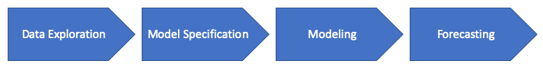
Time Series with Zillow’s Luminaire — Part III Modeling

Time series modeling connects the dots in the starry night; time series forecasting extends the dreams as the breeze brushes the stars into trails. You and I, standing in awe, look at the blue summer night.

In Part I and II of the series “Time Series with Zillow’s Luminaire”, I have walked you through the data exploration and model specification Steps, now we are ready for modeling!

The luminaire offers two main approaches for time series modeling: (A) Kalman Filter modeling and (B) Structural modeling. If this is the first time you've heard of the Kalman Filter, you may not know that numerous devices in our lives have relied on it. The Kalman Filter estimates the trajectory of a moving object. Your iPhone or Android phone has a map app that estimates the location of the phone and driving distance. Cars, fleet trucks, ships, aircraft, or drones have the GPS (Global Positioning System) to track movement with more accuracy. A famous early use was the Apollo navigation computer that took Neil Armstrong to the moon and, most importantly, brought him back.

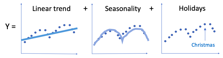
Further, a time series can be considered as the combination of patterns such as a linear trend, seasonality, and holiday effect. So structural modeling (B) tried to model these patterns explicitly.

If you have not read Part I and II of the Luminaire series “Time Series with Zillow’s Luminaire”, I suggest you read them first. In case you found this article first and have not read Part I and II, let me tell you that Luminaire is an open-source product by Zillow for time series forecasting and anomaly detection. You can visit the Luminaire Homepage Luminaire Github or this article Automatic and Self-aware Anomaly Detection at Zillow using Luminaire or this paper.

Bike Share Data

I am going to use the bike share daily data to demonstrate the process, as used in the previous article “Time Series with Zillow’s Luminaire — Part II Optimal Specifications”. Bike-sharing systems are the new version of traditional bike rentals. A user can easily rent a bike from a particular location and return to another location. The bike-sharing daily count is highly correlated to weather conditions and seasonality (day of week and season). The bike share data possess a strong seasonality effect and change point effect, as shown in “Business Forecasting with Facebook’s “Prophet”. The following code first loads the bike share data, plots it, then performs data exploration as done in Part I. The data exploration identifies many change points.

The Jupyter notebook of this article is available for download via this Github link.

Data Exploration

The first step of time series modeling is data exploration, as I explained in Part I: “Time Series with Zillow’s Luminaire — Part I Data Exploration”. So let me just do the same thing:

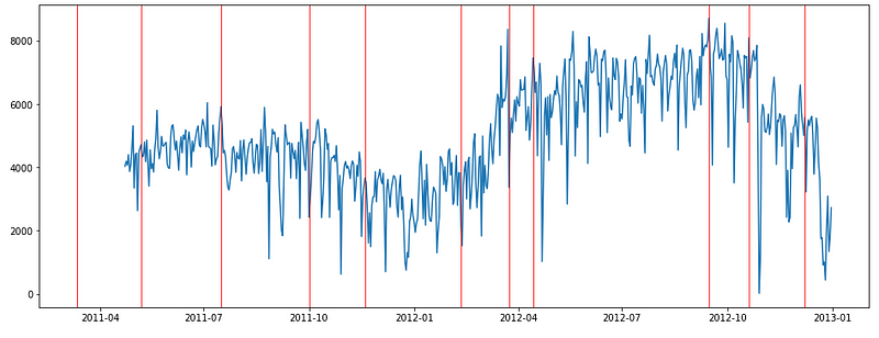
The above reveals the characteristics of the time series such as its frequency, its trend, and the change points. Now let’s move to the model.

(A) Kalman Filter Model

I gave an extensive review of the Kalman Filter in the article “Kalman Filter Explained!”. The Kalman Filter LADFilteringModel in the Luminaire Anomaly Detection (LAD) class is available in this API. I train the model object “lad_filter_obj” and save it as “model”:

I then use the model to test if 2,000 on “2012–06–08” is outside the boundary or not:

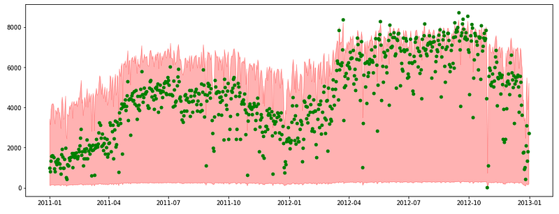
The function score() outputs very rich results as the following. It shows the scoring is successful. The prediction for that day is 2,387 with a standard error of 735.4. The standard error is what we will use to come up with the margin of errors later. It also verifies that the value 2,000 is not an anomaly (“IsAnomaly”= False).

({'Success': True,
  'AdjustedActual': -0.5175304914865355,
  'ConfLevel': 90.0,
  'Prediction': 2387.718712243808,
  'PredStdErr': 735.4123249948354,
  'IsAnomaly': False,
  'IsAnomalyExtreme': False,
  'AnomalyProbability': 0.897174478745516,
  'DownAnomalyProbability': 0.948587239372758,
  'UpAnomalyProbability': 0.05141276062724194,
  'NonStationarityDiffOrder': 1,
  'ModelFreshness': -20.6},
 <luminaire.model.lad_filtering.LADFilteringModel at 0x206bee3b0f0>)

I want to score all the data points and get the confidence intervals. So I developed the following code snippet that scores each data point and appends to the output data “output_pred” iteratively. I define the upper and lower bounds as three standard errors away from the mean prediction.

To plot the actual values (the green dots) and the confidence intervals (the orange area), the following code snippet is developed. You can see some of the green dots are outside the confidence intervals. They can be labeled as outliers.

(B) Structural Model

A time series can have patterns such as an upward or downward trend, seasonality, or holiday spikes. These patterns can be modeled explicitly in a regression-like setting. This modeling approach is called structural modeling. The most common structural approach is the Auto-Regressive Integrated Moving Average (ARIMA), which includes the AR term, the I term, and the MA term. It is noted as ARIMA(p,d,q) that p is the order of the AR term, d is the number of differencing to make the time series stationary, and q is the order of the MA term. I gave more explanation in “A Technical Guide on RNN/LSTM/GRU for Stock Price Prediction”.

Another type of structural modeling is the Seasonal-trend Decomposition (STD) which splits a time series signal into three parts: seasonal, trend, and residue. Along with this approach, the Generalized Additive Model (GAM) is a more flexible form that specifies a long-term linear trend, a yearly seasonal effect, and any holiday effect. See my article “Anomaly Detection for Time Series“ for a detailed treatment.

You can specify if the structural model will include holidays as exogenous variables in the regression, and the order for the Auto-regressive (AR) or Moving-average (MV) component of the model. You can also specify whether to take a log transform of the input data. Click this API for the model specifications or this tutorial of Luminaire. The holidays include the following:

Memorial Day, plus the weekend leading into it
Veterans Day, plus the weekend leading into it
Labor Day
President’s Day
Martin Luther King Jr. Day
Valentine’s Day
Mother’s Day
Father’s Day
Independence Day (actual and observed)
Halloween
Superbowl
Easter
Thanksgiving, plus the following weekend
Christmas Eve, Christmas Day, and all dates up to New Year’s Day (actual and observed)

Every time series has its structural specifications. You can apply the structural model to your time series.

Conclusion

I hope this article gives you a better understanding of this topic. I have made the code in this article available for download via this Github link. If you like to have a comprehensive review, the following sequence will help:

Part 1: “Anomaly Detection for Time Series“
Part 2: “Detecting the Change Points in a Time Series”
Part 3: “Algorithmic Trading with Technical Indicators in R”
Part 4: “Kalman Filter Explained!”
Part 5: “Business Forecasting with Facebook’s “Prophet”
Part 6: “Time Series with Zillow’s Luminaire — Part I Data Exploration”
Part 7: “Time Series with Zillow’s Luminaire — Part II Optimal Specifications”
Part 8: “Time Series with Zillow’s Luminaire — Part III Modeling”
Part 9: “A Technical Guide on RNN/LSTM/GRU for Stock Price Prediction”

Join Medium with my referral link — Chris Kuo/Dr. Dataman

Readers are recommended to purchase books by Chris Kuo:

The explainable AI: https://a.co/d/cNL8Hu4
Transfer learning for image classification: https://a.co/d/hLdCkMH
Modern time series anomaly detection: https://a.co/d/ieIbAxM
Handbook of Anomaly Detection: https://a.co/d/5sKS8bI