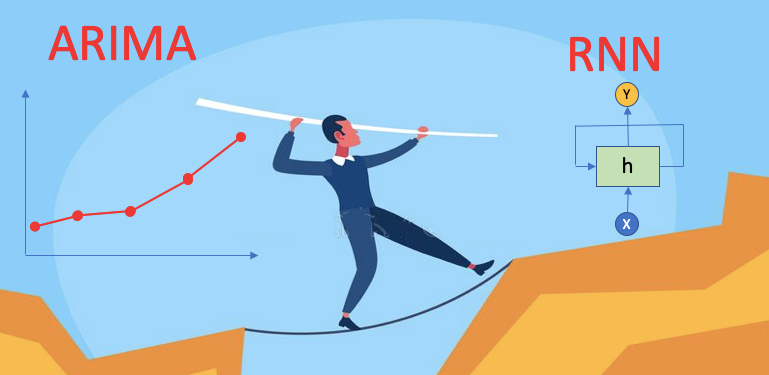
A Technical Guide on RNN/LSTM/GRU for Stock Price Prediction

Sequential data prevail in our lives. Voice data, song data, or language data are examples of sequential data, and univariate time series data are special cases. In sequential data, data arrive sequentially, and the new data should not be abrupt from the previous data. For example, a sentence can be:

• “I am going to feed the dog then do my homework,” or
• “After dinner, they went out for a walk.”

The next word should follow certain grammar rules to its previous word. The serial connectivity is an important property of sequential data. When someone raises an unfinished sentence like “I am going to …”, the hearer expects to hear certain words that can complete the sentence and making grammar sense. For example, it would be obscure if I hear “I am going to I make a ball”, in which the underlined words should not be there. Similarly, a song is a sequential data type. It would be abhorrent if the next musical notes do not follow coherently with the previous notes.

In sequential data, we are interested in forecasting multiple periods in the future. For example, in the sentence “I am going to …”, we are interested in knowing the multiple words after the existing words “I am going to”. We are not just interested in a one-word or one-period forecast.

While modeling sequential data, we need to capture the property on serial connectivity. Serial connectivity between data points implies the influence of a previous data point may appear in a much latter period. Neural Networks have made tremendous contributions in modeling sequential data. They can provide multi-period forecasting capability into the future. Many commercial language translation tools are powered by neural network models that can understand the meaning of a word in certain context and translate instantaneously from one language to another. Such neural networks are powerful in dealing with univariate time series. They can forecast not just one-period ahead but multiple periods in the future.

In explaining the basics of the neural networks in time series, I do not assume that readers should already possess strong knowledge in neural networks. This allows the book to go over the concepts gently. In this and next two chapters, I will explain the Recurrent Neural Networks (RNN), the Long Short-Term Memory network (LSTM), and the Gated Recurrent Units (GRU) models. These three variants of models have wide applications in any sequence-to-sequence data such as language translation modeling or speech-to-text modeling. The Transformer-based models such as [1] or [2] are outside the scope of this article.

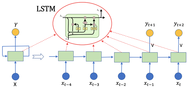
It is not as easy to learn RNN, LSTM, and GRU as we learn regression. In my class, I often feel there is a knowledge gap between regression and deep learning. The variation in terminology also creates a knowledge gap. It takes a lot of preparation to jump too deep learning, and those students jumping successfully may not regress to regression easily (you may like the pun). That’s the motive for me to write “Explaining Deep Learning in a Regression-Friendly Way” to bridge regression and the standard feedforward neural network. In learning RNN/LSTM, you may have seen RNN or LSTM abstract diagrams like Figure (A) but still, feel lost. Part of the obstacle is labeling. I wish these diagrams can label the time series data exactly where they are. In an ARIMA model, we see how Yt, Yt-1, Yt-2, …, produce Yt+1 in a mathematical formula. But how are they represented in an RNN diagram?

I will cover RNN, LSTM, and GRU. After reading this sequence of articles, you will have an in-depth understanding of RNN/LSTM/GRU, and be able to use them to predict stock prices. Do you think it is worth reading? Then grab a cup of coffee and start!

Let me start with some leading questions:

• How univariate time series can be re-organized to fit in a neural network framework.
• The differences between the standard feedforward neural network and an RNN.
• The graph representation of an RNN
• The data requirement for an RNN model

We will uses stock market data to help readers understand the property of serial connectivity. First, the stock price of today should be highly influenced by those of recent days. Second, the price of same day last year may still influence today’s price. The time series seems to have a long memory throughout all its past. Stock price time series deserve continual research effort and innovation. For readers who have just started your research on stock price movement, you may be interested in my articles “Algorithmic Trading with Technical Indicators in R”, “Stock Market Anomalies” and “Stock Market Anomaly Detection” Are Two Different Things, and “Kalman Filter Explained!”. Also, you are likely to develop a web service for your stock price prediction service. You may be thinking of Flask or Django as your web-service frameworks. I highly recommend Streamlit. as I explain in “Building a Stock Market App with Python Streamlit in 20 Minutes” and “Let’s Talk About the Taylor Rule for Monetary Policy”.

Let me mention several data types and how deep learning deals with each data type. Data can be categorized broadly as (1) Multivariate data (In contrast with serial data), (2) Serial data (including text and voice stream data), and (3) Image data. Deep learning has three basic variations to address each data category: (1) the standard feedforward neural network, (2) RNN/LSTM, and (3) Convolutional NN (CNN). For readers who are looking for tutorials for each type, you are recommended to check “Explaining Deep Learning in a Regression-Friendly Way” for (1), the current article “A Technical Guide for RNN/LSTM/GRU on Stock Price Prediction” for (2), and “Deep Learning with PyTorch Is Not Torturing”, “What Is Image Recognition?“, “Anomaly Detection with Autoencoders Made Easy”, and “Convolutional Autoencoders for Image Noise Reduction“ for (3). You can bookmark the summary article “Dataman Learning Paths — Build Your Skills, Drive Your Career”.

The entire notebook is available through this Github link.

(A) A Short Recap of the ARIMA Model

The recursive nature in ARIMA helps readers to understand the recursive nature of RNN. The ARIMA (Auto Regressive Integrated Moving Average) models the recursive nature based on (a) a linear combination of its lags and (b) a linear combination of lagged forecast errors, to forecast the future. ARIMA model includes the AR term, the I term, and the MA term. An ARIMA(p,d,q) model is characterized by three terms:

• p is the order of the AR term
• d is the number of differencing to make the time series stationary
• q is the order of the MA term

Below are two examples:

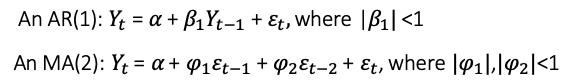
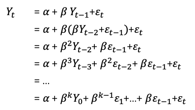
We can consider the AR term as a partial difference. The absolute value of the coefficient on the AR term tells you the percent of a difference you need to take. The above AR(1) tells us Yt is obtained from knowing the value of Yt−1. But Yt−1 is obtained from Yt-2 and so on. Or in other words, data are not uncorrelated. Yt cannot be obtained just by Yt-1 and not by Yt-2. The solution for Yt can be found through recursive substitution:

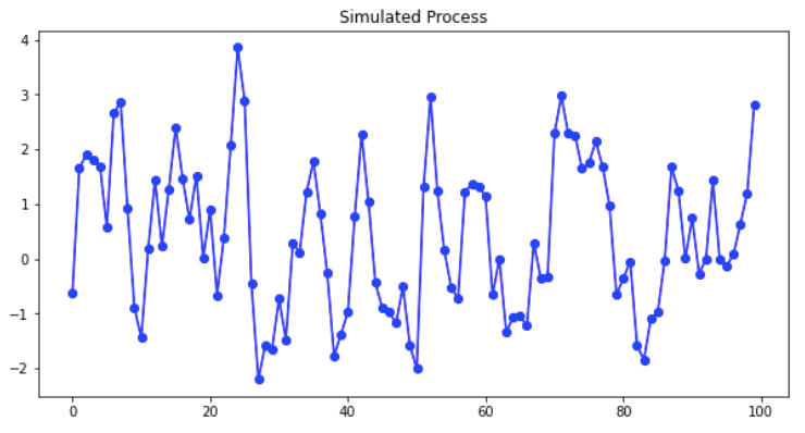
There are many ARIMA tutorials available online such as this one or this. I suggest that interested readers search for relevant tutorials. Below I simulate an ARIMA(2,0,0) for Yt = 0.8 Yt-1–0.2 Yt-2.

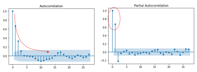
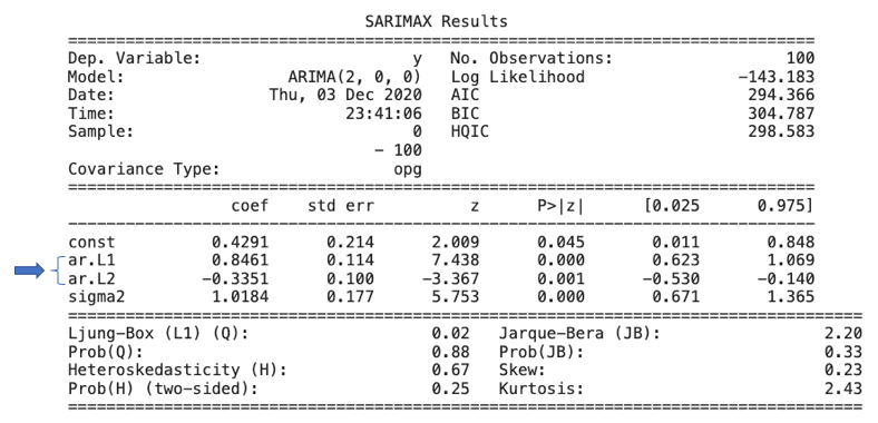
ARIMA models use the autocorrelation function (ACF) and partial autocorrelation (PACF) plots to determine the numbers of AR and/or MA terms. Figure (A.1) shows the ACF gradually tapers to zero, while PACF has two significant spikes. With this suggestion, we can test an AR2 model specification. (For the rules of ACF and PACF, click here for more detail.) Figure (A.2) presents the estimated model coefficients, which are close to those we have specified.

(B) Why Can’t the Feedforward NN Characterize Sequential Data Effectively?

Figure (B.1) shows a standard feed-forward neural network. It has the input layer, the hidden layers, and the output layer. Every neuron is a weighted average of the neurons in the previous layer. The weights are the parameters to be estimated. A neural network is a supervised learning model in which the input layer contains N input values and the output layer has the target value y. Notice that the input values are not connected. They can be uncorrelated. The standard feedforward neural network takes the input data points as independent, without considering the correlations between the input data. This limitation makes the feedforward NN not suitable for modeling sequential data.

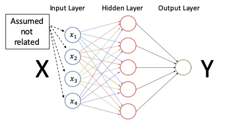
Assume we want to predict the next two periods of a time series. If a standard feed-forward neural network is used, we can let x1, x2, x3, x4 be the past data points, and the target y1, y2 be the values of next two periods. Figure (B.2) shows the structure.

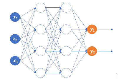
However, the serial connectivity in sequential data posts a special challenge that a standard feedforward NN not able to solve. First, it can only model the current period but cannot handle the serial correlation property in sequential data. In other words, x1, x2, x3, x4 are not serial correlated. Second, it does not have the capacity to memorize previous inputs.

(C) A Recursive Neural Network (RNN)

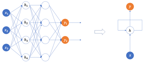
In order to retain the memory of previous inputs, the Recursive Neural Network (RNN) should be specially designed. The outputs of the previous periods should somewhat become the inputs of the current periods. And the hidden layers will recursively take the inputs of previous periods. In the right-hand side of Figure (C) is a simple graph representation of an RNN. The hidden layer receives the inputs from the input layer, and there is a line to connect a hidden layer back to itself to represent the recursive nature. For now, you just need to know there is a recursive nature in the simplified RNN graph. In latter sections, I will explain every element in an RNN graph explicitly.

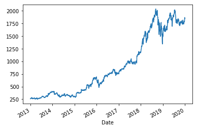
(D) Load the Stock Price Data

We are going to use daily prices from 2013 to 2018 as the training data, and 2019 as the test data.

(E) Re-Organize Data for RNN/LSTM/GRU

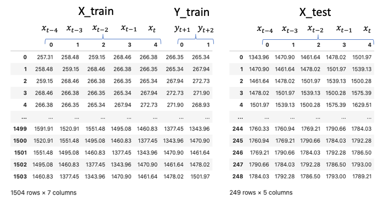
RNNs are supervised deep learning techniques. We will create inputs and targets from a univariate time series for model training. Let me describe the ultimate data structure will be, then I will describe how we get there. The data frames in Figure (E.3) are what we are heading to. There are X_train and Y_train for modeling training, and X_test for predictions. This data structure is unique in modeling a time series in Deep Learning.

In order to get there, there are two popular data structures: many-to-many and many-to-one. The many-to-many uses the values of multiple periods to forecast the values of multiple periods in the future. The many-to-one uses the values of multiple periods to forecast the value of only period in the future.

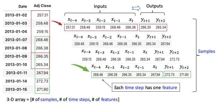
(E.1) Many-to-many

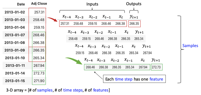
We are interested in using the prices of the past X days to forecast those of the future Y days. For the sake of illustration, let me use the prices of only 5 days to forecast the prices for the next 2 days. There are multiple inputs (5 data points) and multiple outputs (2 data points). This data structure is called many-to-many. Figure (E.1) creates samples from the univariate time series as the red window moves along the series. Each sample has 5 inputs and 2 outputs. Each input of a sample is called the time step, and each time step has one number, called a feature. The number of features can be multiple. For example, if we model both the “Adj. Close” and “Open” prices together in a time step, there are two features. Here we just model “Adj. Close” so the number of features is one.

(E.2) Many-to-one

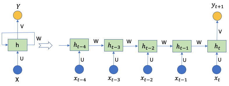
Figure (E.2) shows the case when there is only one output. This is called many-to-one.

(E.3) RNN/LSTM/GRU Requires a 3-D Array as the Inputs

The three dimensions are:

• Tensor: One tensor is a vector that enters the model
• Time Step: One-time step is one observation in the tensor.
• Feature: One feature is one observation at a time step.

The 1-D array above should be converted to a 3-D array =

[# of samples, # of time steps, # of features].

This can be done by using np.reshape(samples, time steps, features). I provide more exercises in the Jupyter notebook through this Github link. You are advised to print out the 3-D arrays in the Notebook available.

(E.3) The Code for Input and Output Data

Below is the code to generate the input and output data in Figures (E.3). There are 1,504 rows or samples in the training data. There are 249 samples in the test data.

I convert the X_train, Y_train, and X_test to data frames and printed them below.

(F) How Does RNN Work?

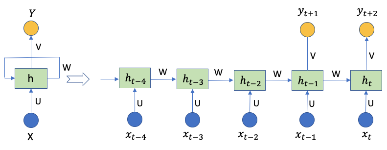
Figure (F.1) shows an RNN and unrolls it to a full neural network. Do you notice it is very different from the feedforward neural network in Figure (B)? RNNs are called recurrent because they perform the same task for every sample, given the outcome from the previous computations. We also can consider RNNs to have a “memory” that passes information from one time step to the next time step. In theory, RNNs can handle a long sample of many time steps. This is suitable for stock prices because the information is passed down from one price point to the next price point. This means the price information of many days ago, or the same day last year still has its residual information to today’s price. However, a long sample makes the computations very time-consuming and may not be necessary. In our case, each sample (row) in X_train has 5 inputs and 2 outputs. So the diagram has 5 steps xt-4, xt-3, xt-2, xt-1, xt, and two output time steps yt+1 and yt+2. The network has 5 hidden layers because there are 5 input time steps.

Step-by-step explanations:

• Xt-4 to Xt: the time steps of a sample, e.g., 257.31, 258.48, 259.15, 268.46, 266.38 in Figure (C.3). Each time step is a vector of the number of features. Our case has one feature, so the dimension for each of xt-4 to xt is 1.
• ht-4 to ht: The hidden state of time step t-1 to t. It’s the “memory” of the network. Each is calculated based on the previous hidden state and the input at the current step:

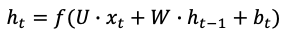
• The first hidden state h0 is typically initialized to zeros.
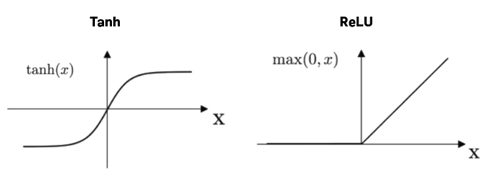
• The activation function f(.) is tanh or ReLU (Rectified Linear Unit). The idea is similar to the logit function in logistic regression. Why does a logistic regression need the logit function? In a linear regression Y = XB + e, the independent variables X and the predicted Y can take any values from negative to positive infinity. Because logistic regression is about probability, we need to transform the output to be between 0 and 1. Otherwise, the output values may explode to negative or positive infinity. To prevent this from happening, here the tanh or ReLU function is applied to transform the output to be between 0 and 1.

• bt: the noise term
• yt+1, yt+2: are the outputs. They are the matrix product of the hidden neurons and the activation function tanh,
• U, W, and V: are the parameter matrix. The same matrix is used repeatedly across all steps. This reflects the fact that we are performing the same task but just with different inputs. What is the dimensionality of the matrix? This is not a trivial question. Let me explain in (D.1).

(G) What Is the Dimensionality in the RNN/LSTM/GRU Layer of Keras?

This is probably the most confusing question. The official Keras’ description for “units” is “dimensionality of the output space”. I still think it is not easy to understand. (Some online sources confuse it with the number of time steps in a sample.) I feel it may be better to name the “units” as “latent dimension” or “latent_dim” (as used in this Keras code). This renaming at least implies that the dimensionality is internal and has nothing to do with the outside parameters.

The dimension of the hidden layer is the “units”. Since there are hidden layers, we need to specify the number of neurons for the hidden layers. The hidden dimension can be any number. The hidden dimensionality determines the capability of RNN to retain the memory for all the past information. It is usually not a small number and is conventionally the multiple of 32, such as 32, 64, or 128.

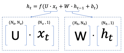
Figure (G) explains the hidden dimensionality. Each time step xt-4 to xt is a vector of the number of features. Our case has one feature, so the dimension for each of xt-4 to xt is 1, i.e., Nx = 1. Nh is the dimension of the hidden layer. If Nh=32, then the parameter matrix U is (32 x 1). The dot product of U and xt has the dimension (32 x 1) x (1 x 1) = (32 x 1). Likewise, the parameter matrix W is (32 x 32), the dot product of W and ht-1 is (32 x 32) x (32 x 1) = (32 x 1). The noise vector therefore should be a (32 x 1) vector.

(H) Build a Simple RNN Model

Tensorflow and Keras are the two most popular platforms for modeling neural networks. TensorFlow is an open-source platform for machine learning. It has many libraries and community resources. It enables ML developers to build and deploy ML applications easily. Keras is an open-source deep-learning API written in Python. It supports Tensorflow or Theano. Big companies such as Microsoft, NVIDIA, Google, and Amazon have contributed actively to Keras’ growth.

The procedure to build the transfer learning model is the same as building any neural network. It involves three steps in Keras: (1) .sequential() to build the model architecture, (2) .compile () to compile the model with the loss function and optimization method, and (3) .fit() to train the model. The function .sequential() defines the structure of a neural network. It is the pipeline to add any layers to a model. Once a model is defined, the compiling step defines the evaluation metric and the optimizer. The last step executes the actual model training.

(H.1) Declare the Model

This step gives the model specification for a simple RNN model.

(H.2) Compile the Model

The second step of building a neural network is the compiling step. This step defines the evaluation metric and the optimizer.

An evaluation metric is the loss function that is used to judge the performance of a model. Keras includes almost all the evaluation metrics. The evaluation metrics belong to three categories: (a) the regression-related metrics, (b) the probabilistic metrics, and © the accuracy metrics. The regression-related metrics include mean squared error (MSE), root mean squared error (RMSE), mean absolute error (MAE), mean absolute percentage error (MAPE), and so on. When your target variable is continuous and you would like to pursue the minimum deviation in terms of percentage errors or absolute errors, you should consider the regression-related metrics.

The probabilistic metrics are considered when your prediction is a probability. They include binary cross-entropy and categorical cross-entropy. If your target is binary, you can use binary cross-entropy. If your target is multi-class, categorical cross-entropy.

The accuracy metrics calculate how often predictions equal labels. The frequently-used metrics are the accuracy class, binary accuracy class, and categorical accuracy class. As the name suggests, the binary accuracy class calculates how often predictions match binary labels, and the categorical accuracy class calculates how often predictions match multiple labels.

The optimizer is a function that optimizes a model. Optimizers use the above loss function to calculate the loss of the model and then try to minimize the loss. Without an optimizer, a machine learning model can’t do anything.

The popular optimizers include the Stochastic Gradient Decent (SGD), RMSprop, Resilient Back Propagation (RProp), the Adaptive Moment (Adam), and the Ada family. The SGD is probably the most widely used optimizer. The RMSprop maintain a moving average of the gradients and uses that average to estimate the variance. The RProp is widely used in multi-layered feed-forward networks. The Adam is considered more efficient and requires less memory when working with a large amount of data and parameters. It requires less memory and is efficient. I use rmsprop as the optimizer.

(H.3) Fit the Model

The third step is the training step. This is a time-consuming step. You will see “epoch 1”, and “epoch 2” appearing on your screen.

In this step, we deal with a unique concept in a neural network called “epoch”. In an epoch, the model goes through all data exactly once. The model parameters are updated in each epoch until they reach optimal values.

If you specify too many epochs, the model will commit overfitting. It will learn the training data too well but predict poorly for a new dataset. How do we determine the optimal number of epochs? The answers are the loss and accuracy metrics. When a model is trained with more epochs, the loss will decrease, and the accuracy will increase. After a certain number of epochs, the loss will stop decreasing but increase, and the accuracy decreases. It indicates the model training should end with that epoch.

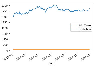
The model prediction is terrible! Do you know why? This is because the input data were not normalized. In (D.2) we will normalize the input data. The key takeaway is: that normalization is necessary for RNN/LSTM/GRU. The function actual_pred_plot() also calculates the mean square error. The result is 3,072,268.

Notice that you can add several simpleRNN layers as shown but commented out in the code. You can test their performances.

(I) Normalized Data Are Needed for RNN/LSTM/GRU

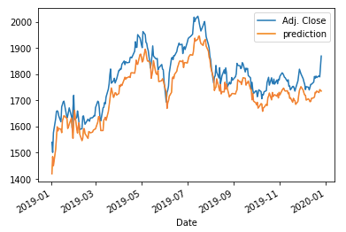
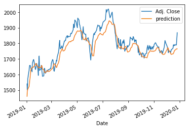
The code below (Line 16–19) normalizes the input data. When you standardize data to train your model, remember that only the training data are used to fit the scaler transformation, then the scalar is used to transform the test input data. Do not scale x_train and x_test independently, as I documented in “Avoid These Deadly Modeling Mistakes that May Cost You a Career”. Line 72 applies the scalar to convert the scaled predictions to the original scale. The prediction performance is much better as shown in the graph. The MSE is 3,852.

(J) Why Do We Need LSTM/GRU?

The optimizer of RNN gets the first-order derivative of the loss function to search for the optimal values. Because RNN is recursive, the first-order derivation process will make a number smaller and smaller, then eventually vanish. This is called gradient vanishing. This certain mathematical process makes RNN not a good choice to retain memories. We need a recursive structure so that the information does not vanish quickly. This is the motive for LSTM and GRU. (For readers who may not be familiar with the optimization process: A loss function is a metric that measures the errors between the actual and the predicted values. An optimizer is an algorithm that changes the weights of the neurons to pursue the minimum error. A popular optimizer is the Stochastic Gradient Descent (SGD). The article “My Lecture Notes on Random Forest, Gradient Boosting, Regularization, and H2O.ai” gives a detailed description of SGD. The above code specifies RMSprop, Root Mean Square Propagation, as the optimizer.)

(K) Why LSTM (Long Short-Term Memory)?

Hochreiter and Schmidhuber (1997) proposed the LSTM structure to retain memory for RNNs over longer periods. It solves the problem of gradient vanishing (or gradient explosion) by introducing additional gates, input, and forget gates. These additional gates can control better over the gradient, enabling what information to preserve and what to forget. These gates are sigmoid functions with output in [0,1] to pass limited information or all information. A value of zero means filtering out the information completely, while a value of one means passing the information completely. The structure is called Long Short-Term Memory because it uses the short-term memory processes to create longer memory. (So do not mislabel “Long Short-Term Memory” as “Long-Short Term Memory”.)

How does LSTM retain the memory of a long time ago? LSTM has its layers called the cell state, often labeled Ct, in addition to the hidden layers to prevent the old information from vanishing too soon. In our stock price example, the price of this Friday may be influenced by the prices of previous Fridays, or even the price of the same day last year. RNNs may not be able to retain the price information of the same day last year, while LSTM in theory is designed to retain it.

(K.1) Math Explanation for the Issue of Vanishing Gradients

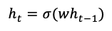
Feel free to skip the mathematical explanation and jump to (F.2) if you already get the idea. Assume we have a hidden state ℎ𝑡 at time step 𝑡 to make the math simple, we remove the bias bt and the input xt terms:

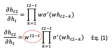
Taking the first-order derivatives we get the following equations. The circled coefficient vector is the key. It will vanish exponentially to zero, or explode exponentially to infinity.

To overcome the problem, LSTM adds the cell state 𝑠𝑡. The derivative equation is:

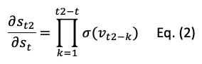
Here 𝑣𝑡 is the input to the forget gate. Because there is no decaying factor w, it does not vanish so fast. However, you may ask that Eq. (2) also has the sigmoid function, so the matrix multiplication also will make the values vanish. You are correct. LSTM still will suffer the problem of vanishing gradients, but not as fast as Eq. (1).

(K.2) The Structure of LSTM

Many papers demonstrate only the internal structure of LSTM — this may still leave you confused about how the system works. Thus I draw a complete diagram of LSTM in Figure (F.2), similar to that of RNN in Figure (D.2), to show you the whole system.

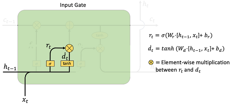
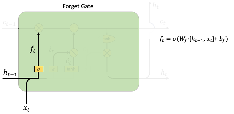
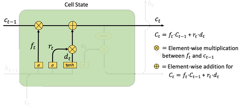
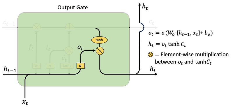
The LSTM has four components: input gates, forget gates, cell state, and output gates.

• Input Gate: the goal is to take in new information xt. There are two functions to take in new information: rt and dt. The rt concatenates the previous hidden vector ht-1 with the new information xt., i.e., [ht-1, xt], then multiplies with the weight matrix Wr, plus a noise vector br. The dt does something similar. Then rt and dt are multiplied element-wise to get the cell state ct.

• Forget Gate: The forget gate ft looks very similar to rt in the input gate. It controls the limit up to which a value is retailed in the memory.

• Cell State: it calculates an element-wise multiplication between the previous cell state Ct-1 and forget gate ft. It then adds the results from the input gate rt times dt.

• Output gate: Here ot is the output gate at time step t, and Wo and bo are the weights and bias for the output gate. The hidden layer ht either goes to the next time step or goes up to output as yt. In the following code Line 12, yt is obtained by applying another tanh to ht. Note that the output gate ot is not the output yt, it simply is the “gate” to control the output.

(K.3) LSTM Code

(K.4) LSTM With Regularization

Overfitting is a serious sin in machine learning. When you train a model on your training data and apply it to the test data, the accuracy of the test data usually is less than that of the training data. We know this is because the model has fitted the training data too well, including the noises in the training data. However, if overfitting just makes your prediction for the test data less effective, what’s the big deal? Why do academia and practitioners devote decades of work to prevent overfitting?

The real issue is that overfitting not only makes your model inefficient, but it could also make your prediction very wrong. Suppose your final model has ten variables, eight of which capture the real patterns and the other two variables, noises. In other words, the two variables overfit noises and are useless. Suppose you are going to predict new data with your ten-variable model, and suppose the new values for the two variables are large. Guess what will happen? Your prediction will be very wrong due to the two variables and the large values in the new data. So overfitting does not just make your model ineffective, it can make your prediction very wrong.

Deep learning uses the dropout technique to control overfitting. The dropout technique randomly drops or deactivates some neurons for a layer during each iteration. It is like some weights are set to zero. So in each iteration, the model looks at a slightly different structure of itself to optimize the model. See “Explaining Deep Learning in a Regression-Friendly Way” for more detail.

Handling dropout in RNN/LSTM/GRU is also a research topic. In a feedforward neural network, dropping neurons is easier because there is no connectivity between neurons of the same layer. However, in RNN/LSTM/GRU, dropping time steps harms the ability to carry informative signals across time. What are the remedies? Pham et al. (2013) suggest applying dropout only between layers in deep-RNNs and not between sequence positions. Gal and Ghahramani (2015) suggest applying dropout to all the components of the RNN (both recurrent and non-recurrent) but retaining the same dropout mask across time steps. This paper provides a good review.

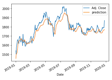
The MSE is 2,152.

(L) GRU (Gated Recurrent Units)

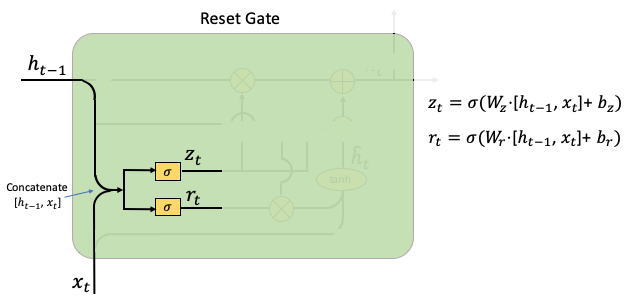
The GRU was invented by Cho et al. (2014) in a company with RNN and LSTM. It is expected more variations of the recursive network will continue to emerge. GRU also aims to solve the vanishing gradient problem. GRU does not have the cell state and the output gate like those in LSTM. It, therefore, has fewer parameters than LSTM. GRU uses the hidden layers to transfer information. GRU calls its two gates the reset gate and the update gate. Let me explain them one by one.

(L.1) The Structure of GRU

The parameters of GRU include Wr, Wz, and W. The reset signal rt determines if the previous hidden state should be ignored while the update signal zt determines if the hidden state ht should be updated with the new hidden state hat(ht).

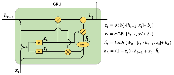
• Reset Gate: This achieves what the input gate and forget gate of LSTM achieve. The gate rt determines if the previous hidden state should be ignored. The gate zt is generated for the update gate with hat(ht). Wz and Wr are the weight parameters to be trained, bz and br are the noise vectors.

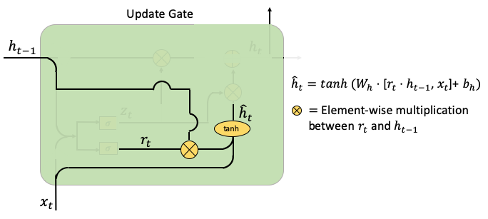
• Update Gate: (Part 1) This part multiplies rt and ht-1. The multiplication means how much of ht-1 will be retained or ignored. This creates a temporal hat(ht) to be used for the update of ht. Wh and bh are weight parameters and the noise vectors.

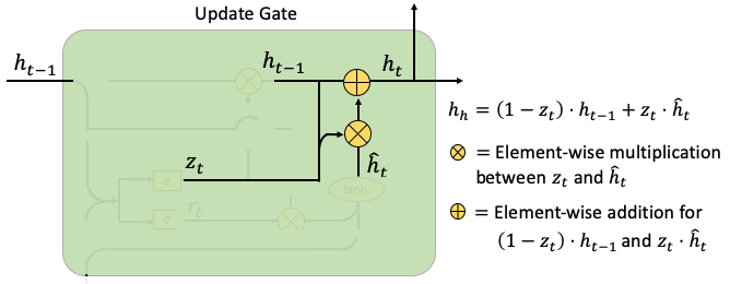
• Update Grade: (Part II) This part computes the weighted average between ht-1 and hat(ht), according to the weight zt. If zt is close to zero, the past information contributes little and new information contributes more.

(L.2) GRU Code

(L.3) GRU with Regularization

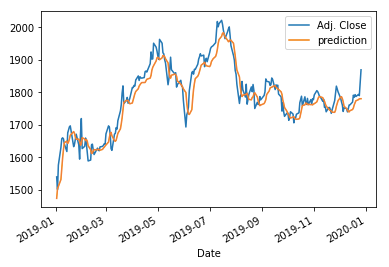
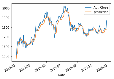
The following code applies the dropout technique to GRU. Because it is very similar to the above, I am not going to describe it too much. The MSE is 1,232.

References

• [1] Vaswani, A., Shazeer, N., Parmar, N., Uszkoreit, J., Jones, L., Gomez, A. N., Kaiser, Ł. & Polosukhin, I. (2017). Attention is all you need. Advances in Neural Information Processing Systems (p./pp. 5998–6008)
• [2] Chien, C., & Chen, K.Y. (2022). A BERT-based Language Modeling Framework. INTERSPEECH.

Readers are recommended to purchase books by Chris Kuo:

• The explainable AI: https://a.co/d/cNL8Hu4
• Transfer learning for image classification: https://a.co/d/hLdCkMH
• Modern time series anomaly detection: https://a.co/d/ieIbAxM
• Handbook of Anomaly Detection: https://a.co/d/5sKS8bI