Explaining Deep Learning in a Regression-Friendly Way

Often deep learning or neural network is presented in their category with their jargon. Learners are oriented with brain-like anatomy to “imagine” how deep learning can function in the context of the brain. Learners are presented with neurons, interconnectivity, and a complex system of neural networks. In my lecture’s transition from regression to deep learning, I somehow feel there is a moment of silence — like jumping over a deep gap. It takes a lot of preparation to jump to deep learning, and those students jumping successfully may not regress to regression easily (you may like the pun). The variation in terminology also creates a knowledge gap. This post tries to present deep learning with a regression-friendly approach. I will explain neurons, activation function, layers, optimizers, and so on. I will show you how to build a logistic regression in a deep-learning framework. Once you have a good understanding, I will take you deep into:

L1 and L2 Regularization in deep learning, and
Dropout regularization in deep learning.

The goal of this article is not just to build a deep learning model to perform the job of logistic regression. That will be overkill. The goal is to explain in great detail so you can build more complex deep learning models. After reading this post, you will be comfortable with deep learning modeling. I also recommend you the sister article “A Technical Guide on RNN/LSTM/GRU for Stock Price Prediction”.

Regarding the platform, Keras and PyTorch have gained massive popularity in the past few years among others such as MXNet. Keras is a high-level Python wrapper for the low-level libraries TensorFlow and Theano. This article walks you through Keras to build the models. If you want to explore PyTorch, I recommend my previous post “Deep Learning with PyTorch Is Not Torturing”, which walks you through gently how to build deep learning models with PyTorch. In addition, I have written a series of articles on deep learning or neural network. See “What Is Image Recognition?“, “Anomaly Detection with Autoencoders Made Easy”, and “Convolutional Autoencoders for Image Noise Reduction“. You can bookmark the summary article “Dataman Learning Paths — Build Your Skills, Drive Your Career”.

The entire notebook can be downloaded at this Github.

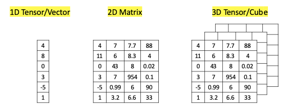
(A.1) Input Data Are Called “Tensors” in Deep Learning

In a Y = XB + e regression formula, Y is an 1-dimension vector, and X is a 2D matrix. The input dataset is called a data frame. A data frame can contain numerical values, categorical or text values.

In deep learning, the input data are called tensors. Had you known a “tensor” means nothing but a one-dimension vector, you would feel relieved. Why don’t they just call it “vector”? I don’t know. Where does this unusual term come from? It came from the Latin tensor, meaning “that which stretches”. The study of materials stretching under tension is the study of the tensors. A mathematician named Woldemar Voigt (1898) borrowed this term for a vector of numbers. A Tensor is a 1D vector. A data frame is a 2D matrix or a 2D tensor. Imagine an EXCEL spreadsheet that has one column Y, and many columns together called X. The one-column Y is a 1D tensor, and the X is a 2D tensor.

An important reminder is that deep learning models can interpret only numeric data. If a data frame has categorical data, you will need to convert them to numeric values through one-hot encoding or other encoding methods. The post “A Data Scientist’s Toolkit to Encode Categorical Variables to Numeric” provides a comprehensive list of encoding methods.

Image data also needs to be transformed into an n-dimensional tensor. This post does not plan to cover image data. Readers interested in image data transformation are advised to reference “Deep learning with PyTorch”, “What Is Image Recognition?“, “Anomaly Detection with Autoencoders Made Easy”, and “Convolutional Autoencoders for Image Noise Reduction“.

(A.2) The Neurons in the Input Layers are the Input Variables

For regression learners, the term neuron in a neural network is foreign and the term layer is daunting. However, you probably have seen many neural network diagrams like Figure (A) below. So let me introduce this network step by step. The diagram is a model. How do we understand a model? Regression is a framework that models the relationship between X and Y. A decision tree is a framework that models the relationship between X and Y. So Figure (A) is a neural network diagram that models the relationship between X and Y. A neural network model has one input layer, one output layer, and the hidden layers. You assign the predictor X to the input layer, and the target Y to the output layer to train the model. If there are no hidden layers, the neural network only has the input layer and the output layer. This simplest form becomes a logistic regression, as I am going to show you in later sections.

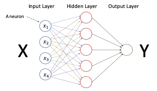
How about the nodes in the network? They are called neurons. The neurons in the input layer are the easiest to understand. A neuron in the input layer is a variable. The X matrix in Figure (A) has 4 variables, so it has 4 neurons (or 4 columns/vectors/tensors). If there are 100 input variables, there will be 100 neurons in the input layer. Also, remember a neural network model can only accept numeric values. If there are 80 numerical variables and 20 categorical variables each with 10 categories, the number of neurons in the input layer will be 80 + 20 x 10 = 280 neurons (or 280 columns/vectors/tensors).

(A.3) Neurons in the Hidden Layers

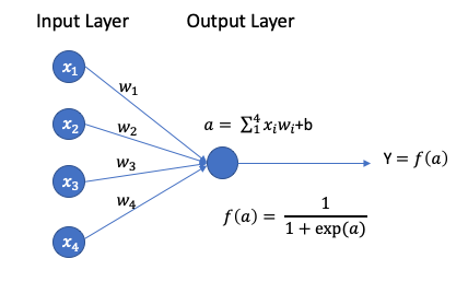
A neuron receives inputs from the neurons in the previous layer. Each neuron is a weighted sum of ALL the data values in the previous layer, or say, each neuron is a linear combination of the values in the previous layer. The weights are the parameters of the model to be trained as w1-w4 in Figure (B) below. Just like the parameter vector B in Y= XB + e is the solution for a regression model, these weights w1-w4 are the secret sauce of the model.

(A.4) The Activation Function

We are almost there to building a logistic regression using the neural network framework. But there is one more component called the activation function. It works like the logit function in logistic regression. Why does a logistic regression need the logit function? In a linear regression Y = XB + e, the independent variables X and the predicted Y can take any values from negative to positive infinity. Because logistic regression is about probability, it’s not possible to achieve such output with a linear regression model and we need to transform the output to be between 0 and 1.

Sigmoid function: So similar idea applies to the neural network. The range of the output value would explode to negative or positive infinity. To prevent this from happening, the neural network applies a sigmoid function as shown in the left panel below, to transform the output to be between 0 and 1.

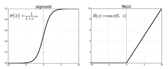
ReLU function: Another popular activation function is the ReLU (rectified linear unit), which is shown in the right panel. It converts any negative value to zero. I will describe this in more detail at the end of the article.

(B.1) Load the Boston Housing Data

I chose a popular dataset the Boston housing data. This dataset documents the median house values with several attributes. The housing price medv is the median value of owner-occupied homes in $1000s. I create a binary target variable “Y” = 1 if the house value is above the median, or otherwise 0. This data frame has 506 rows and 14 columns. I arbitrarily chose the following six predictors for illustration purposes:

CRIM: per capita crime rate by town.
ZN: proportion of residential land zoned for lots over 25,000 sq. ft.
RM: average number of rooms per dwelling.
AGE: proportion of owner-occupied units built before 1940.
DIS: weighted mean of distances to five Boston employment centers.
LSAT: lower status of the population (percent).

Standardization: The code above also scales the input variables. Notice that only the training data are used to fit the scaler transformation, then the scaler is used to transform the test input data. A common mistake of novice learners is to scale x_train and x_test independently. This is a deadly sin that you want to avoid. In the article “Avoid These Deadly Modeling Mistakes that May Cost You a Career” I document the common mistakes in data science. If you are interested, take a look.

Deep Learning does not make the normality assumption. To run a standard linear regression, people make the following assumptions:

The relationship between X and Y is linear
Errors are normally distributed
Homoskedasticity of errors (or, the equal variance around the line).

These assumptions are not required in a deep learning model.

(B.2) Let’s Build a standard Logistic Regression

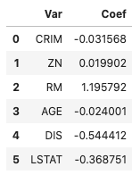
The mean squared error is 0.1068. For your reference, the coefficients are

(C) Let’s build in Deep Learning:

A neural network is much more general than logistic regression, so it can cover a logistic regression. We can think of logistic regression as a special case of a neural network.

There are three core ideas in a neural network: (1) layers are stacked sequentially, (2) neurons do the computation, and (3) an activation function is used in each layer to bind the outcome. These three processes correspond to the Keras classes Sequential, Dense, and Activation, as shown in Figure (C).

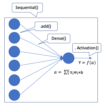
Sequential Declare an empty model that we are going to stack layers. See Line 3 in the code below.
add() Add a layer.
Dense(1,input_dim=6) The dense layer is where the computation happens. It performs a matrix multiplication (dot product) plus a noise vector. It is called the “dense” layer because it compacts every possible connection between the neurons of the previous layer and the current layer. The values used in the matrix are the weights that can be trained and updated with the help of back-propagation (to be explained later). In this example, there is one neuron in the current layer, and 6 input neurons in the previous layer. So the syntax is Dense(1, input_dim=6). See Line 4.

Activation(activation='sigmoid')): This applies the sigmoid function to produce Y. Notice that Line 4 and 5 can be combined into one line of code as shown in Line 8.

We are done with the model specification for a deep learning model to perform what a logistic regression does. The model will be trained using the optimizer compile() and fit(). The model results in [‘loss’, ‘mean_squared_error’] = [0.1031, 0.1031]. The MSE is the same as that of logistic regression.

(E) Optimizers

What is a loss function and what is an optimizer? A loss function is a metric that measures the errors between the actual and the predicted values. An optimizer is an algorithm that changes the weights of the neurons to pursue the minimum error. A popular optimizer is the Stochastic Gradient Descent (SGD). The article “My Lecture Notes on Random Forest, Gradient Boosting, Regularization, and H2O.ai” gives a detailed description of SGD. The above code specifies RMSprop, Root Mean Square Propogation, as the optimizer.

You may ask a fundamental question: “why regression does not use an optimizer such as SGD to find the optimal parameters, but machine learning techniques need it?” The reason is that regression can derive its optimal solutions analytically or in a closed-form equation. The loss function is differentiable. However, not all loss functions are differentiable to derive a trackable solution. So numerical methods such as SGD or Newton’s Method are used to get the optimal solution.

The above lines of code are the core lines of a basic neural network. These basic code lines can be extended to a very complex form. I will use the following example to experiment with the model.

(F) Add More Layers to the Deep Learning Model

You can add any number of layers and neurons to the above basic neural network. Below I experiment with two hidden layers:

Line 4: the first hidden layer has 4 neurons.
Line 5: the second hidden layer, has two neurons. Notice the additional layers do not require you to specify the number of neurons in the previous layers.
Line 6: the output layer.

[‘loss’, ‘mean_squared_error’] = [0.1121, 0.1121]. When you add more layers, the model is likely to yield a better result, even overfitting the data. In a Generalized Linear Model (GLM) we can apply L1 or L2 regularization to control overfitting. How can we regularize a neural network model to mitigate overfitting? In short, there are two methods. First, a neural network can use regularizers.l1() or regularizers.l2() for L1 and L2 regularization. Second, the neural network can use dropout() regularization. If you are not familiar with L1 or L2 regularization, please check “My Lecture Notes on Random Forest, Gradient Boosting, Regularization, and H2O.ai”.

(G) Standardize Data for a Better Model Performance

For a classification modeling problem, it is a good practice to standardize the data before modeling. This usually yields model performance. The code below is the same as the above, except it builds on the standardized data. The results seem better than the above results: [‘loss’, ‘mean_squared_error’] = [0.0981, 0.0981].

(H) Attack Overfitting

Overfitting is a serious sin in machine learning. When you train a model on your training data and apply it to the test data, the accuracy of the test data usually is less than that of the training data. We know this is because the model has fitted the training data too well, including the noises in the training data. However, if overfitting just makes your prediction for the test data less effective, what’s the big deal? Why do academia and practitioners devote decades of work to prevent overfitting?

The real issue is that overfitting does not just make your model inefficient, it could make your prediction very wrong. Suppose your final model has ten variables, eight of which capture the real patterns and the other two variables, noises. In other words, the two variables overfit noises and are useless. Suppose you are going to predict new data with your ten-variable model, and suppose the new values for the two variables are large. Guess what will happen? Your prediction will be very wrong due to the two variables and the large values in the new data. So overfitting does not just make your model ineffective, it can make your prediction very wrong. That’s why we focus so much on attacking overfitting. If you are familiar with these techniques, your technical competency in data science will greatly increase.

(I) L1, L2 Regularization & Dropout Regularization

Regularization adds a penalty term to the loss function to penalize a large number of weights (parameters) or a large magnitude of weights. Deep learning offers LASSO (L1) and RIDGE (L2):

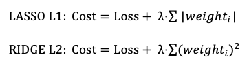
Besides L1 and L2, deep learning also has Dropout regularization. You are advised to test the L1, L2, and Dropout regularization in your deep learning models.

(I.1) L1

The above code sets 𝜆 = 0.01. The results are: [‘loss’, ‘mean_squared_error’] = [0.09434, 0.09434].

(I.2) L2

The above code sets 𝜆 = 0.01. The results are: [‘loss’, ‘mean_squared_error’] = [0.09841, 0.09841].

(I.3) Dropout Regularization

The dropout technique randomly drops or deactivates some neurons for a layer during each iteration. It is like some weights are set to zero. So in each iteration, the model looks at a slightly different structure of itself to optimize the model.

The above code sets the dropout rate at 0.25, meaning 25% of the neurons are to be dropped out. The results are: [‘loss’, ‘mean_squared_error’] = [0.0974, 0.0974].

(J) How to Understand the Complexity of a Neural Network Model?

Regression is considered complex if it has many parameters. Likewise, deep learning is complex if it has many weight parameters to train.

Let me show you two models to see which model is more complex (more weighting parameters). Suppose a binary classification problem has 200 columns/variables and 1 billion rows. The 200 variables refer to 150 numerical and 50 categorical variables. Each of the 50 categorical variables has 400 levels. There are two models:

Model 1: 3 hidden layers with 300 neurons each.
Model 2: 1 hidden layer with 500 neurons

Let’s compute the number of weightings for each model and compare. In general, we multiply the number of neurons in adjacent layers, then add up all the pairs. In this question, the categorical variables must be one-hot encoded to be a separate neuron. So the 50 categorical will be transformed to 50 x 400 = 2,000 dummy variables. We have a total of 150 + 2,000 = 2,150 input neurons. The output has 1 neuron.

Model 1: 2150 x 300 + 300 x 300 + 300 x 300 + 300 x 1 = 825,300
Model 2: 2150 x 500 + 500 x 1 = 1,075,500

So Model 2 is more complex.