My Lecture Notes on Random Forest, Gradient Boosting, Regularization, and H2O.ai

There are many articles teaching machine learning techniques. Why read this one? This article describes the most common machine learning concepts and techniques with depth and breadth. After reading, you will be able to demonstrate nice machine learning in H2O, and convince your audience of your technical decisions for your models.

(A) What Does Ensemble Mean in Machine Learning?

In a musical ensemble, there are all kinds of instruments like flutes, oboes, clarinets, bassoons, trumpets, violins, violas, cellos, bass violas, drums, and keyboards. These base instruments compose a grand concert. In machine learning, ensemble methods are supervised machine learning techniques that combine several base models to produce one optimal predictive model. Ensemble methods have produced better predictive performance compared to a single model, proven in many machine learning competitions such as the Netflix Competition, KDD, and Kaggle.

It is worth mentioning that in real life many classification problems are multi-class. If you ever face the need to model a multi-class problem, see my post “A Wide Variety of models for Multi-class Classification”.

(B) Two Types of Ensemble Methods — Bagging & Boosting

The term Bagging comes from Bootstrap Aggregating. It builds many models independently and then averages their predictions. The best-known example is the random forest technique. The random forest method builds many decision trees and then takes the average for the outcomes of all the decision trees.

In contrast, the Boosting method fits many small models sequentially to reduce the error. It first builds a small model and calculates the residual error between the actual and the prediction. The error will be large, but no problem. In the second round, it aims at the residual error from the first round and builds a small model to reduce it. In the third round, it takes the previous residual error as the target and builds another small model to reduce it. This goes on and on until the residual error is reduced to zero. Once you aggregate all these small models, the predictability of the collective models delivers superior results. These small models are called weak learners. The superpower is not in each small model but in in the special process — it attacks the error sequentially until the error is close to zero. The best-known example is the gradient boosting technique.

Either bagging or boosting method, the aggregated model is usually better than any single model.

(C) Let’s Revisit a Single Decision Tree

We exercise the decision-tree thinking process in our daily life. So it became popular right after it was innovated. Suppose a person is deciding if to play golf outside or not. He considers many conditions such as sunny or rainy, humid, or windy. He also considers if going with a friend or not, aiming for the tournament or not, costly or not, and so on. Figure (I) draws out his thought process.

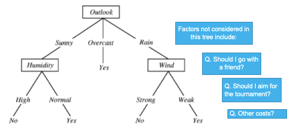
Suppose in the past this person always considers similar questions. There is a lot of past data and his outcomes (the target). We can build a decision tree on the past data to find patterns to predict his next decision.

A decision-tree model has its weaknesses. It only fits the past data once and it can fit that particular data too well. These issues result in overfitting. That’s why the ensemble comes to play. Rather than just relying on one decision tree, the ensemble methods sample multiple times and make a final predictor based on the aggregated results of the decision trees.

(D) How Does Random Forest Work?

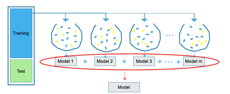
The random forest technique draws some samples to build a model, draws some samples again to build another model, and so on. All of these sampling and modeling is done independently and simultaneously as shown in Figure (II). The outcome is the average of the predicted values of all the models.

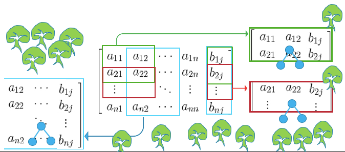
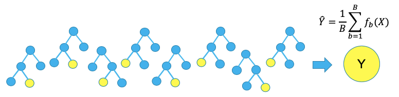
Let me use a mathematical way to illustrate this approach. Figure (II) shows a matrix of features and the target in columns. Every time it takes some rows and some columns with the corresponding target rows to build a tree model. The number of rows or columns can be large or small. The same samples can be drawn repeatedly at different times as well. We try to build a large tree model each time. When you have many trees, you get a forest. Because the trees tend to be large, they are prone to overfit each drawn sample. But no problem. The outcome is the average of the predicted values of all the trees. So it tends to even out the overly fitted prediction. Figure (III) shows how it averages the predicted values to get the final prediction.

(E) How Does Gradient Boosting Work?

Gradient boosting has long and stark development literature (Freund et al., 1996, Freund and Schapire, 1997, Breiman et al., 1998, Breiman, 1999, Friedman et al., 2000, Friedman, 2001). It builds many small models like decision trees to reduce the residual errors from the previous round sequentially. This iterative process is what “Boosting” means. It also relies on an optimization algorithm called the “gradient descent”.

What Is Gradient Descent?

The Stochastic Gradient Descent, Gradient Descent, or called SGD, is probably the most popular optimization algorithm. Gradient descent is a first-order iterative optimization algorithm for finding the minimum.

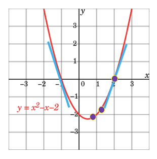
How do you find the optimal x value that minimizes the parabola function y=x²-x-2? If the function is tractable, all you need to do is to set the first-order derivative to zero: dy/dx=2x-1=0. This is the same as saying the slope is zero at x=1/2. Tractable in mathematics means there is sufficiently operationalizable to allow a mathematical calculation toward a solution.

But not all the functions are tractable, and mostly not. In this case you can use a numeric approach to search for the optimal value that minimizes the target function. It starts with any randomly picked number on the parabola. Let’s do some math step by step to see how it approaches the optimal value.

• Suppose it is x=3. At that point, the slope and y values are dy/dx=2x-1=2∗3–1=5 and y=4 respectively. The value of the slope is positive, meaning as x increases y will increase.
• Let’s take another random x on the parabola. Suppose it is x = -3, the slope and y value are dy/dx=2x-1=2∗(-3)-1=-7 and y=10 respectively. The derivative tells us we are getting closer or away from the minimum.
• Since we want to minimize y, it should go in the opposite direction. That’s why it is called “descent”. You can have a gradient ascent if it is in the same direction.
• We set the iteration in Equation (1) such that the next x is the current x minus the slope. The ⍵ is the step length or called the learning rate (lr). It can take any value. A small ⍵ value means every step is a small step, which takes a longer time to approach zero.

In summary, the gradient boosting method builds many small models (weak learners) sequentially. In each iteration, it uses the gradient descent algorithm

(F) The Bias and Variance Trade-off

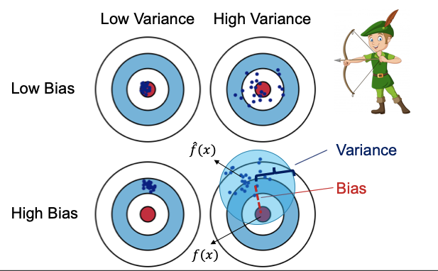
Suppose you played archery on a nice Sunday afternoon. Some of your shots got the bullseye and some didn’t. A geek like me sat observing your practice. Then he came up with a weird mathematical observation: “Do you know there is no way to achieve both zero bias and zero variance at the same time?”

“What?”, you asked. (You had no idea where this guy came from.) The geek got excited and proceeded: “Bias is how far the average of your shots away from the bullseye. Variance is how close the multiple shots are to each other.” He draws four targets as below. (Haven’t you met any geek that you have to give some time to and wish him to finish soon?) “There are four possibilities, the best one is low-bias and low-variance and the worst one is high-bias and high-variance.” “This I know,” you replied. Then he said something surprising to you: “If you want to reduce the bias, the variance increases. There exists a trade-off between bias and variance. This is the famous bias and variance trade-off.”

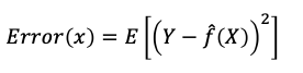
“Interesting,” you said politely. He didn’t get it and said: “Suppose Y is the actual value and f(x) is the prediction, let’s define the error as the expected value of the squared difference between the actual and prediction like the following:

With some mathematical deduction, he came up with the following relationship. The error term consists of the bias and the variance and an irreducible error term.

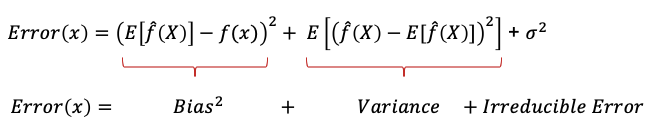
However, there exists a trade-off between bias and variance. You cannot decrease both to zero. Figure (IV) demonstrates the trade-off: when bias goes down, the variance inevitably goes up.

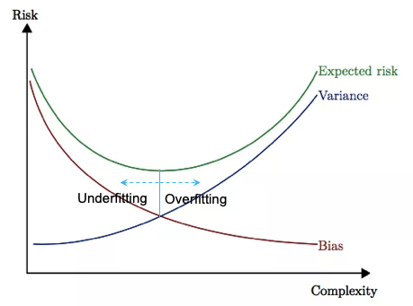
Overfitting happens when a model learns the data too well including background noises. A model that delivers a small bias may include too many variables and has over-fitted the data. The trade-off is inevitable: a model either (a) has a large number of variables or (b) a large magnitude of coefficients, or both.

(G) Regularization Is Needed to Prevent Overfitting

Overfitting is a serious sin in machine learning. When you train a model on your training data and apply it to the test data, the accuracy of the test data usually is less than that of the training data. Your instructor explains that your model could have fitted the training data too well, including the noises in the training data. However, if overfitting just makes your prediction for the test data less effective, what’s the big deal? Why do academia and practitioners devote decades of work to prevent overfitting?

The real issue is that overfitting does not just make your model inefficient, it could make your prediction very wrong. Suppose your final model has ten variables, eight of which capture the real patterns and the other two variables, noises. The two variables overfit noises and are useless. Suppose you are going to apply your ten-variable model to new data, and suppose the new values for the two variables are large. Guess what will happen? Your prediction will be very wrong due to the two variables with large values. So overfitting does not just make your model ineffective, it can make your prediction very wrong. That’s why we focus so much on attacking overfitting. If you are familiar with these techniques, your technical competency in data science will greatly increase.

There are two approaches to mitigate an overfitting problem. One is the Data validation approach like train/test split, 10-fold cross-validation, or leave-one-out cross-validation. Another one is Regularization (LASSO, Ridge, Elasticnet). To help you master the content easier, here let me explain regularization first. I will explain the data validation approach in Section (I).

Regularization adds a penalty term to the loss function to penalize a large number of coefficients or a large magnitude of coefficients.

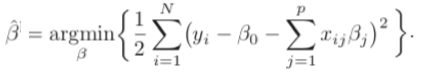
Let’s start with the standard multivariate linear regression model without regularization. Below is the loss function or the Sum of Squared Error (SSE):

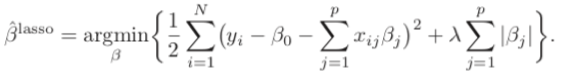
LASSO (Least Absolute Shrinkage and Selection Operator) — L1

Overfitting occurs when there are more parameters than needed. So why won't we penalize the model if there are too many parameters? This is the idea of the LASSO regularization. It simply adds the sum of the absolute value of coefficients to the loss function SSE (as shown below). Here λ ≥ 0 is a parameter that controls the amount of shrinkage: the larger the value of λ, the greater the amount of shrinkage. If 𝜆=0, LASSO becomes the above standard function. LASSO is also known as the L1 regularization. How do we remember “L1” or “L2”? A good way to remember “L1” is “1” which looks like the symbol for the absolute value.

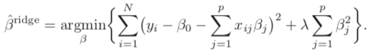
RIDGE — L2

if overfitting arises when the total magnitude of the coefficients is too large, why don’t we penalize the model when the magnitude is large? This is the idea of the RIDGE regularization. It adds the sum of the squared value of coefficients to the loss function SSE. It “amplifies” the magnitude of a parameter by squaring its value so the model will be sensitive to a large parameter value (in absolute value). How do we remember “L2”? A good way to remember “L2" is the “2” in the “squared” terms in the equation.

Jerome Friedman Trevor Hastie once said: ”Ridge regression is known to shrink the coefficients of correlated predictors towards each other, allowing them to borrow strength from each other.”

• In the extreme case of k identical predictors, the variables each get an identical coefficient with 1/kth. LASSO, on the other hand, tends to pick one and ignore the rest.
• Ridge reduces the magnitude of coefficients close to zero; in contrast, LASSO reduces the magnitude of coefficients exactly to zero. Therefore LASSO works like a feature selector that picks out the most important coefficients.

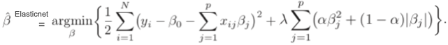
ElasticNet

Overfitting occurs if (a) there are too many parameters, or (b) large magnitude, or both. The LASSO and RIDGE techniques each address some aspects (note that the two situations will not be mutually exclusive), why don’t we use both LASSO and RIDGE? That’s the idea of ElasticNet. Zou and Hastie (2005) introduced the ElasticNet penalty. The elastic net selects variables like the LASSO, and shrinks the coefficients of correlated predictors like RIDGE:

(H) GBM vs. XGBoost vs. LightGBM

GBM does not have regularization so it is prone to overfitting. To correct this issue, Tianqi Chen and Carlos Guestrin presented the XGBoosting (EXtreme Gradient Boosting) that incorporates the regularization formalization in the loss function. It uses block structure to support parallelization in tree construction and the ability to fit and boost new data added to a trained model. It can efficiently reduce computing time and allocate optimal usage of memory resources. Important features of implementation include the handling of missing values (Sparse Aware).

LightGBM

Microsoft developed the LightGBM to be a “fast, distributed, high-performance gradient boosting framework based on decision tree algorithms, used for ranking, classification, and many other machine learning tasks.” It is designed to be distributed and efficient with the following advantages:

• Faster training speed and higher efficiency.
• Lower memory usage.
• Better accuracy.
• Support for parallel and GPU learning.
• Capable of handling large-scale data.

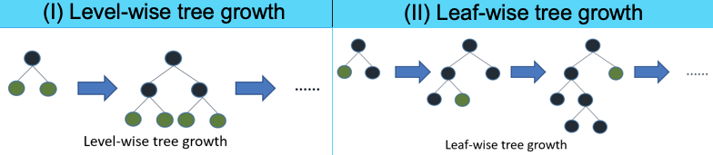
How does the LightGBM improve its accuracy? It uses the “leaf-wise” algorithm to achieve a higher level of accuracy. Figure (VII) explains what leaf-wise means. The leaf-wise tree grows on single branches to achieve precision. It could be very deep in a branch. In contrast, the level-wise tree tries to grow branches of the same level before moving to the next level. It looks more balanced.

The leaf-wise tree growth is likely to over-fit when the data size is small. So you are advised to use parameter max_depth to limit the depth of tree <=3.

(I) Modeling in H2O

As said in the beginning, H2O has proven to be one of the favorite tools of many data scientists. It streamlines modeling development and production and can produce models that can be run in other languages such as Java. Below is an excerpt from the official H2O.ai website:

H2O is a fully open-source, distributed in-memory machine-learning platform with linear scalability. H2O supports the most widely used statistical & machine learning algorithms including gradient-boosted machines, generalized linear models, deep learning, and more. H2O also has an industry-leading AutoML functionality that automatically runs through all the algorithms and their hyperparameters to produce a leaderboard of the best models. The H2O platform is used by over 18,000 organizations globally and is extremely popular in both the R & Python communities.

I am going to use the red wine quality data on Kaggle.com. I use the same dataset in my post “Explain Your Model with the SHAP Values” and “Explain Any Models with the SHAP Values — Use the KernelExplainer” so you can compare. The input variables are the content of each wine sample including fixed acidity, volatile acidity, citric acid, residual sugar, chlorides, free sulfur dioxide, total sulfur dioxide, density, pH, sulphates, and alcohol. There are 1,599 wine samples. Below I create a binary target variable “quality_bin” for the modeling.

Below I will show you how easy it is to use H2O to produce (I.1) Random Forest, (I.2) GBM, (I.3) XGB, (I.5) GLM without regularization, (I.6) GLM with regularization, (I.7) Deep Learning, and finally (I.8) automatic ML. To simplify, I make no effort in optimizing the models. Readers shall pursue the optimal training results when applying to your projects.

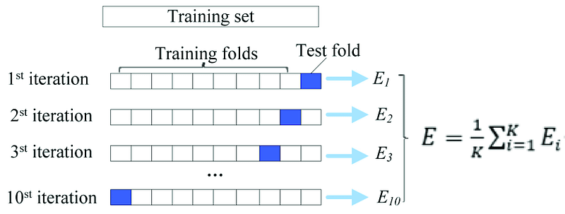
It is worth mentioning I will use the 10-fold cross-validation (CV) in the following code. For readers who may not be familiar with the 10-fold CV, here I give a gentle illustration. In the typical 70% train/30% test split, you build the model using the 70% training data and validate the model using the 30% test data. But your model is validated only once so is still subject to potential overfitting. The 10-fold CV goes beyond the typical approach. It splits the data randomly into ten equal subsets. In the 1st iteration, it reserves one subset to be the test data and the rest nine subsets to be the training data. It builds a model using the nine subsets and computes the prediction error on the test data. In the 2nd iteration, it reserves another subset to be the test data and the rest nine subsets to be the training data. It builds a second model using the training data and computes the prediction error on the test data. There will be ten models and ten prediction errors. The performance measure is the average error of the ten prediction errors. This approach can be computationally expensive but does not waste too much data.

(I.1) H2O Random Forest (RF)

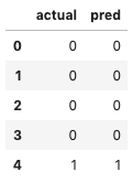
Let me make the following function to put together the actual and predicted values. Because all the H2O prediction outcomes follow the same format (except GLM, which I will explain later), the code snippet will make our lives easier.

And here is the Area-under-the-curve (AUC):

We got AUC = 0.8795.

(I.2) H2O Gradient Boosting Machine (GBM)

(I.3) H2O Extreme Gradient Boosting (XGB)

(I.4) H2O Generalized Linear Model without Regularization

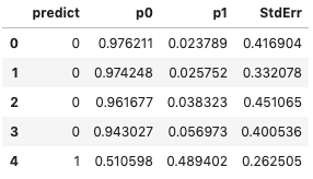
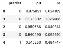
The GLM predict() outputs the above four columns. ‘p1’ is the predicted probability for the target. You want to take ‘p1’. ‘p0’ is merely 1-p1. With the threshold, the ‘predict’ is obtained from ‘p1’ into ‘1’ and ‘0’. You can choose different thresholds. H2O uses the thresholds that optimize the F1 score. For more information, see this H2O explanation.

We got AUC = 0.7666.

(I.5) H2O Generalized Linear Model with Regularization

We got AUC = 0.7731.

(I.6) H2O Deep Learning

(I.8) H2O Automatic Machine Learning (AutoML)

The above code snippets show a high level of repetition. Wouldn’t it make sense to write code to train all algorithms, rank by their performances, and then choose the best? This is the motivation for autoML.

The default automatic ML algorithms include Random Forest, Extremely-Randomized Forest, a random grid of Gradient Boosting Machines (GBMs), a random grid of Deep Neural Nets, and a fixed grid of GLMs, and then train two Stacked Ensemble models at the end. For more hyper-parameters, please reference the H2O manual.

To help you implement these code snippets, I put all of them in the following code block:

References

[Freund et al., 1996, Freund and Schapire, 1997] Invent Adaboost, the first successful boosting algorithm

[Breiman et al., 1998, Breiman, 1999] Formulate Adaboost as gradient descent with a special loss function

[Friedman et al., 2000, Friedman, 2001] Generalize Adaboost to Gradient Boosting in order to handle a variety of loss functions.