A Wide Variety of Models for Multi-class Classification

Many real-life examples involve multiple selections. Rather than the “to be” or “not to be” by Hamlet, the choice may be multiple like “Yes”, “No”, “I don’t know”, and “I don’t want to choose”.

Since we use data science to help our lives, we often need to predict an outcome that has multiple options. The good thing is there are many algorithms to perform this job. In this article, I want to show you at least nine popular algorithms to model a multi-class problem. In addition, I want to provide a handy notebook so you can apply it to your data science projects. I organize each method with two sub-sections: (i) Python code, and (ii) the algorithm highlight. This lets you focus on the code part, or the algorithms if you are already familiar with one of them. The nine algorithms are:

• Multinomial/Multi-class Logistic Classification,
• Decision Tree,
• Random Forest,
• Naïve Bayes (NB),
• Gaussian Mixture Model (GMM),
• K-nearest Neighbors (KNN),
• Discriminant Analysis
• Support Vector Machine (SVM), and
• Neural Network (NN).

I will perform the above models on the same dataset in Python. The Python notebook is available via this link.

(0) Let’s Use a Data Example

I use the California house price dataset. This dataset contains information collected by the U.S Census Service concerning housing in California. This dataset can be obtained from the StatLib repository or the scikit-learn datasets. The target variable is the median house value for California districts, expressed in hundreds of thousands of dollars ($100,000). There are 20,640 records with eight numeric columns.

• MedInc: median income in block group
• house: median house age in block group
• AveRooms: average number of rooms per household
• AveBedrms: average number of bedrooms per household
• Population: block group population
• AveOccup: average number of household members
• Latitude: block group latitude
• Longitude: block group longitude

To make the target a multi-class target, I convert the continuous target variable to four classes: (1) ≤100k, (2) 100k~160k, (3) 160k~240k, and (4) 240k+. (Related to the California house price dataset is the Boston house price dataset, which I used to demonstrate Quantile Regression techniques in the post “A Tutorial on Quantile Regression, Quantile Random Forest, and Quantile GBM”.)

Besides the standard training and test split, I do not do any special treatment for the eight numeric columns. This helps to shorten the article to focus on the algorithms.

(1) Multinomial/Multi-class Logistic Classification

A binary logistic regression is the most popular algorithm for predicting binary classes. It predicts the probability of occurrence of a binary event utilizing a logit function. However, it is not designed to model a target with multiple classes. To model a multi-class classification problem, a natural extension is to convert the multi-class target into one-hot variables and fit a standard logistic regression model on each one. In our four-class example, there will be four one-hot columns. This is the multinomial logistic regression which uses the softmax function. I will explain the softmax function later.

(1.1) Python code

• Line 4: lets you specify the regularization part. Regularization is almost always necessary in machine learning modeling to mitigate the issue of overfitting. If you are not familiar with Ridge, LASSO, or Elasticnet regularization, you can take a look at my post “My Lecture Notes on Random Forest, Gradient Boosting, Regularization, and H2O.ai”.
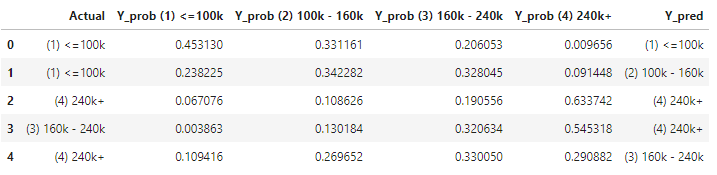
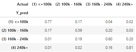
• Line 7–11: uses the function predict_proba() of scikit-learn to provide the probabilities for each of the four classes, or uses the function predict() that produces the maximum predicted class (“Y_pred”). See below.

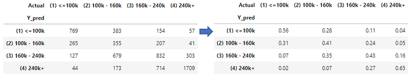
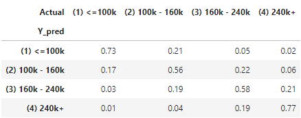
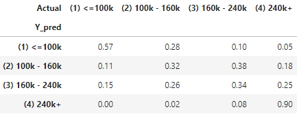
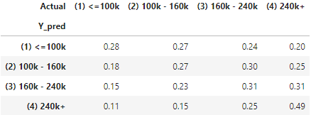
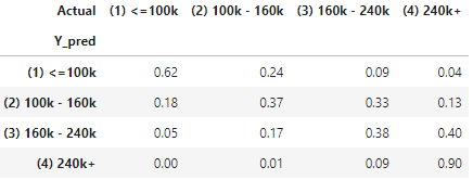
I create the count statistic of Actual vs. Prediction. The count statistic is converted to row percentage to show the prediction accuracy. For those that predicted as “(1) ≤100k”, 56% are “(1) ≤100k”, 28% are “(2) 100k-160k”, and 11% are “(3) 160k-240k” and only 4% are “(4) 240k+”.

(1.2) The Algorithm Highlight

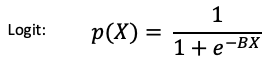
The logit function models the probability of occurrence of a binary event as shown below, where p(x) is the probability of an event, B is the vector of coefficients, and X is the independent variable matrix:

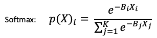
The softmax function extends the two-class logistic function to multiple classes. The word softmax comes from “maximum arguments of the maxima” (abbreviated argmax). It finds the smooth approximation of one-hot argmax. In other words, it finds the argmax for each class (one-hot) of the multiple classes. Formally, let K be the number of classes i = 1, …, K of the target variable, and X be the matrix of the independent variables. The probability for Class i is:

Multinomial logistic regression (LR) is also known by other names such as multinomial logit (mlogit), polytomous LR, multi-class LR, and softmax regression.

(2) Multi-class Decision Tree

A decision tree works naturally with a multi-class target, so it is somehow redundant to call a decision tree a “multi-class decision tree”. However, here I name it “multi-class” just want to emphasize that it can work with a target with multiple classes.

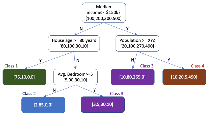
Let me use a hypothetical decision tree to show you the idea. Assume the counts for [Class 1, Class 2, Class 3, Class 4] are [100,200,300,500] as shown in the root node on top of the tree. A decision tree is a series of questions. A decision tree evaluates the variable that best splits the data. The final nodes are where predictions are made. In this hypothetical tree, the green end node has [75,10,0,0]. The maximum count of 75 indicates the green end node is Class 1. Do you notice the count of the true Class 1 in the root node is 100? This means 75 out of 100 Class 1 are rightly labeled as Class 1, and the rest 25 counts are misclassified to other classes. Also, there are 10 Class 2 misclassified as Class 1.

(2.1) Python code

(3) Multi-class Random Forest

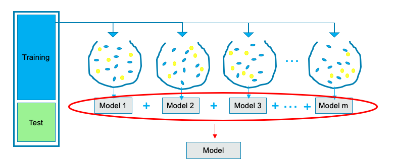
A decision-tree model has its weaknesses. It may overfit a particular dataset. That’s why the ensemble comes to play. Rather than just relying on one decision tree, the random forest technique draws many random samples to build many decision trees. All of these sampling and modeling is done independently and simultaneously as shown below. The outcome is the average of the predicted values of all the models

As explained in (1.1), a tree-based algorithm is natural to model a multi-class classification problem. Since the random forest inherits the tree-based algorithm, it is suitable for modeling a multi-class classification problem as well.

(3.1) Python code

In (1.1) I explained each step. To save code for all the following methods, I create a function Prediction() to do prediction.

(3.2) Algorithm Highlight

Two points about the random forest algorithm worth mentioning: (i) its inheritance to model a multi-class classification problem, and (ii) its mitigation on overfitting. Since I have explained the first one, below let me say a few words about the second one.

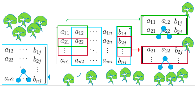
The graph below shows a matrix of features and the target in columns. Every time the random forest algorithm takes some rows and some columns with the corresponding target rows to build a tree model. The number of rows or columns can be large or small. The same samples can be drawn repeatedly at different times as well. Because the trees tend to be large, they are prone to overfit each drawn sample. The outcome is the average of the predicted values of all the trees. So it tends to even out the overly fitted prediction.

(4) Naïve Bayes (NB)

The Naive Bayes model is based on the Bayes theorem. It involves two parts: “Naive” and “Bayes” and let me explain both.

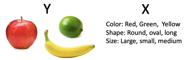
“Bayes theorem”: Some students may be scared by the mathematical representation of the Bayes theorem. However, do you know that we exercise Bayes thinking almost every day? Let me use an example. Below are three classes of fruits (Y): apple, lime, and banana. Let the features of the fruits (X) be “color”, “shape”, and “size”. The features of the fruits are:

• An apple is “red”, “round”, and “large”;
• A lime is “green”, oval”, and “small”, and
• A banana is “yellow”, “long”, and “medium”.

Now if we observe a fruit with the features “red”, “round”, and “large”, can we tell what it is? Yes, we can identify it as an apple with a 100% chance, and 0% chance for lime or banana.

In a classification problem, we observe the features (X) given a class (Yi). We then build a model to predict (Yi) if certain features (X) are observed. This reversal can be easily solved by the Bayes theorem. Eq. (1) shows the Bayes theorem, and Eq. (1.1) shows the names “prior” and “posterior”. Prior is the probability of the fruits. It is our prior information or beliefs in a single probability value. The posterior is p(Yi|X), which is the product of the likelihood, the prior, and the evidence.

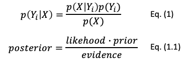
The Bayes theorem describes nicely the predictive thinking. In a predictive problem, we observe p(X|Yi), and we want to predict p(Yi|X). This is exactly the concept of the Bayes theorem.

“Naive”: The X is multivariate, i.e., X = x1, x2, …, xn. Thus the p(Y|X) should be written as the joint probability of x1, …, xn, see this Wikipedia. However, the joint probability quickly becomes intractable. To make the equation mathematically tractable, we make a “naive” assumption that all the features X’s are independent of each other. Then the joint probability of all the X’s because the product of x1, …, xn. Because of this strong assumption, the Bayes classifier is called the Naive Bayes classifier.

(4.1) Python code

(4.2) Algorithm Highlight

It is worth mentioning that the scikit-learn library offers several types of distributions for Naïve Bayes:

• Bernoulli: If your features are mostly binary (1 vs. 0), you can consider the Bernoulli NB.
• Multinomial: If your features are discrete counts you can consider this distribution. Your features may not just be binary (1 vs. 0), but the “count”. Let’s use a text classification problem. Features can be “if a word occurring or not”, or “count of a word occurring in the document”. The former follows a Bernoulli distribution and the latter follows a multinomial distribution.
• Categorical: If your features are mostly discrete, they are better characterized by a categorical distribution. A categorical distribution is a generalized Bernoulli distribution that the possible results of a random variable are one of K's possible categories.
• Gaussian: If most of your features follow a normal distribution, you may consider Gaussian NB.

(5) Gaussian Mixture Model (GMM)

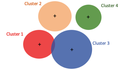
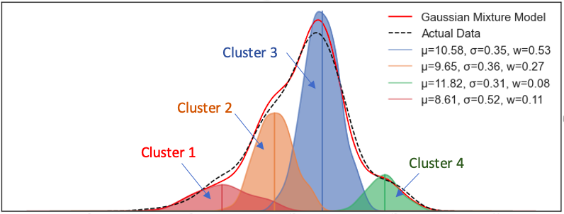
Data usually do not uniformly distribute but cluster together. GMM assumes that the data points are a mixture of data clusters that follow different Gaussian distributions of mean standard deviation. Figure 5A shows four classes, which are labeled as Cluster 1 to 4. GMM gives a fresh look. It interprets the four classes as if they come from four different Gaussian distributions, as shown in Figure 5B.

If the parameters (𝛍, 𝛒) of the four distributions are known, it is easy to guess the distribution that a data point comes from. For example, in Figure 5B the red distribution is on the left. If we observe a data point on the left, we know it is very likely coming from the red distribution. For example, a data point on the left may be described as 90% from the red distribution on the left, 5% from the orange distribution, 3% from the blue distribution, and 2% from the green distribution on the right. Isn’t that the solution for a multi-class classification problem?

However, the parameters (𝛍, 𝛒) of the four underlying Gaussian distributions are latent, which means not observable. Even so, we can use an algorithm called Expectation-Maximization (E-M) to derive the parameters of the latent distributions. I will explain the E-M algorithm later.

(5.1) Python code

If the target has n classes, GMM considers the data are a mixture of n Gaussian distributions with different parameters. In Python code, n is defined by n_components.

(5.2) Algorithm Highlight

The algorithm of GMM is called Expectation-Maximization, or EM. The EM algorithm renders the results in two steps (E-M):

• The E-step: An initial “guess” to assign a posterior probability p(Yi|X). Given the guess, it computes the likelihood function p(X|Yi).
• The M-step: The likelihood function is maximized by choosing the optimal parameters. The new parameters are fed to the E-step to assign a posterior probability again.

The E-step and M-step will repeat iteratively until convergence.

I have covered much of the details in my post “Top Data Science Interview Questions and Answers”. If you are interested in GMM, please take a look.

(6) K-nearest Neighbors (KNN)

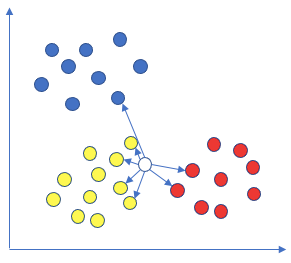
KNN assumes that similar data are nearby of each other. If an unknown data point is close to a class, it is like to be that class. So I would call it the “birds-of-the-same-feather” algorithm. As you see in the graph below, will you call the unknown data point yellow or red, or blue? In the K-data point vicinity, there are four yellow data points, two red points, and 1 blue data point. This unknown data point is likely to be yellow. Do you see it as multi-class in nature?

(6.1) Python code

(6.2) Algorithm Highlight

The algorithm goes like this:

• “K”-nearest neighbors: define a number K for the data points.
• Distance: Calculate the Euclidean distance between the point and all points.
• Ranking: Rank the neighboring points by distance in ascending order
• Voting: use the majority rule to determine the class of the unknown data point. In our example there are 7 data points, 4 are yellow, 2 are red, and 1 is blue. So the unknown class is predicted to be yellow.

How to determine the K? The KNN algorithm is prone to overfitting, especially a small value for K. To overcome the issue of overfitting, the conventional wisdom is to run several KNN models with K=10, 20, …, and 100. You then take the average of the predictions of these KNN models. This will smooth out the outliers. Please read my post “Anomaly Detection with PyOD”.

(7) Linear Discriminant Analysis (LDA)

As the name “linear” suggests, LDA is a linear model for classification and dimensionality reduction. LDA has been in statistics for a long time. It was first formulated by Fisher in 1936 for a binary problem, and later in 1948 generalized by C.R Rao for a multi-class problem. LDA is a supervised classification technique. A noticeable distinction of LDA is that its dependent variable is categorical. Let’s see how it works.

(7.1) Python code

(7.2) Algorithm Highlight

Let me explain the intuition of LDA with a two-class example. The X-axis is a variable (such as HouseAge in our example) in the multivariate problem. This variable can separate the data points into two classes. So one criterion is to find a variable to maximize the distance between two classes. This is called the “Between class”. It can be mathematically formulated as the difference between two class means. On the other hand, we also want the points of the same class to cluster together, which means the data points of the same class should not be too far from its class mean. So LDA formulates the following two criteria:

• Maximizing the between-class distance: (u1 — u2)
• Minimize the within-class distance: (x — u1) or (x-u2)

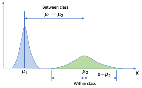
The above two criteria can be formulated as the variance Sb for “between-class” and Sw for “within-class”, where there are n observations and k classes.

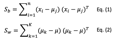
Now the idea is to maximize Sb and minimize Sw. If we put the two together, we are maximizing the ratio of Sb to Sw like Eq. (3). This optimization equation becomes the discriminant function. Isn’t that elegant?

It is important to mention the assumptions of LDA:

• Each feature follows a Gaussian distribution.
• Each of the classes has identical covariance matrices.

(8) Support Vector Machine (SVM)

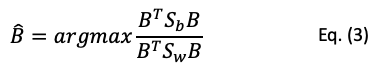
SVM is a supervised machine learning algorithm. In a binary classification problem, it finds the optimal boundary between the two classes. The figure below shows the idea. It finds a hyperplane that maximizes the separation of the data points in a higher dimensional space. The data points with the minimum distance to the hyperplane are called Support Vectors.

Can SVM be extended to multi-class classification problems? Yes. Below let me show you the code, then I will explain how it works.

(8.1) Python code

(8.2) Algorithm Highlight

To make SVM available for a multi-class classification problem, we have to break down the multi-classification problem into multiple binary classification problems. There are two ways: one is called the One-to-One approach, and the second one is the One-to-Rest approach.

• One-to-one approach: This approach forms the multiple classes of the target as pairs of classes. So if a target has three classes Y1, Y2, and Y3. The pairs of classes will be “Y1 vs. Y2”, “Y2 vs. Y3”, and “Y3 vs. Y1”.
• One-to-Rest approach: Similarly if a target has three classes Y1, Y2, and Y3. The pairs of classes will be “Y1 vs. Rest”, “Y2 vs. Rest”, and “Y3 vs. Rest”.

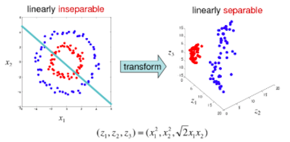
SVM maps the original data to a higher dimensional space to find the hyperplane. Where does intuition come from? Why are data points more separable in a higher-dimensional space? This has to go back to the Vapnik-Chervonenkis (VC) theory. It says mapping into a higher dimensional space often provides greater classification power. The graph on the left shows the blue and red dots can not be separated using any linear transformation. But if all the dots are projected onto a 3D space, the result becomes separable. Isn’t this amazing? For readers who like to understand more, please see my post “Dimension Reduction Techniques with python”.

(9) Neural Network

A standard Neural network (or deep learning) is inherently suitable to model a multi-class classification problem. It predicts the probabilities of multiple classes of a target variable. Below is an image borrowed from my post “What Is Image Recognition?” that explains a neural network can take an image and tells its probability to be a dog, fish, or car. Note that the probabilities sum up to 1.0.

Let’s see how we can apply neural networks here.

(9.1) Python code

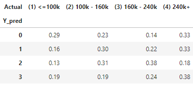
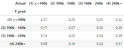
The following statistic of Actual vs. Prediction shows the Neural Network renders very comparative ed results when compared with other models. However, this may vary by subject and data and you are advised to test all the models on your data.

(9.2) The Algorithm Highlight

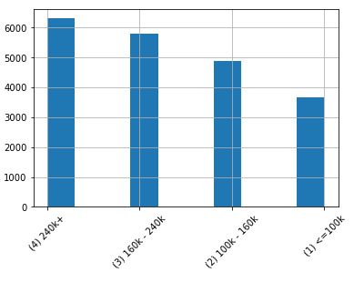
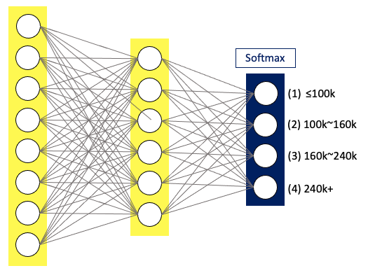
In (1.2) I explained the softmax function. The softmax function is used as the last activation function to normalize the output of a network to a probability distribution. The graph below shows the probability distribution of the four outcomes in our data example.

If you feel unfamiliar with neural networks, I suggest my series of articles on this topic. I often feel there is a learning gap between regression and neural networks or deep learning. So I wrote a post to fill in the gap. If you also feel so, you may be interested in reading my post “Explaining Deep Learning in a Regression-Friendly Way”. There are many variations of neural networks for different types of data. If we categorize data types, we at least can identify three broad data categories:

• (1) Multivariate data (In contrast with serial data),
• (2) Serial data (including time series, text, and voice stream data), and
• (3) Image data.

Deep learning has three basic variations to address each data category:

• (1) the standard feedforward neural network,
• (2) RNN/LSTM, and
• (3) Convolutional NN (CNN).
• (1) “Explaining Deep Learning in a Regression-Friendly Way”,
• (2) “A Technical Guide for RNN/LSTM/GRU on Stock Price Prediction” and
• (3) “Deep Learning with PyTorch Is Not Torturing”, “What Is Image Recognition?“, “Anomaly Detection with Autoencoders Made Easy”, and “Convolutional Autoencoders for Image Noise Reduction“ for (3).

Conclusion

Thank you for reading. I hope this post has given you a better understanding of the topic. The Python notebook is available via this link.