
Top Data Science Interview Questions and Answers

You receive a data science interview opportunity from your dream company. You have surveyed many the-top-50-question types of articles but still feel uncertain. Since there are already many similar articles, why do I dare to add an article to this crowded topic? In this article, I re-write many ordinary answers so a short answer can shine. I hope this approach will help your interview.
Answer with the “What — So what — Now What” Formula
An interviewer would like to probe the breadth and depth of a candidate on a topic. This formula prepares you to provide a thorough answer or at least intent to. It lets you articulate
- What the answer is (80%),
- What it can do and what the advantages or disadvantages are (20%).
You do not need to answer every question with the “what — so what” formula. Some of the questions in this article are worded in a specific way that the formula cannot apply.
I group the questions into machine learning, statistics & probability. Many of these questions and answers are drawn from dataman’s articles. So I also provide the reference for those who are first time seeing the topic or want to understand more.
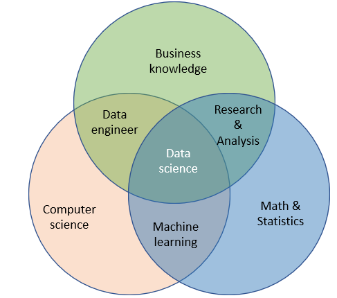
Q. What is data science?
[What] Data science unifies statistics, machine learning, data engineering, and research methods to collect data from various data sources and visualizes information.
[So what] So it can communicate the insights to guide sound, data-driven business decisions.
[Machine Learning]
Q. Name a few alternative measures to the mean square error (MSE). Comment on their advantages and disadvantages.
[What] The mean squared error (MSE) is the average of the squared values of the errors. The errors are the differences between the actual values and the predicted values. The squaring is needed to make a negative value positive because a predicted value can be higher or lower than the actual value. It also gives more weight to larger differences.
Besides MSE, the popular alternatives are mean absolute deviation (MAD), mean squared deviation (MSD), mean percentage deviation (MPE), and mean absolute percentage error (MAPE).
[So what]
- Because MPE or MAPE shows the mean error as the percentage of the actual value, it is preferable by business managers.
- MSE, MAD, and MSD are scale-dependent, while MPE and MAPE are not. For example, if the scale is in thousand or in million, the MSE will be different. In contrast, MPE and MAPE are ratio statistics so are not scale-dependent.
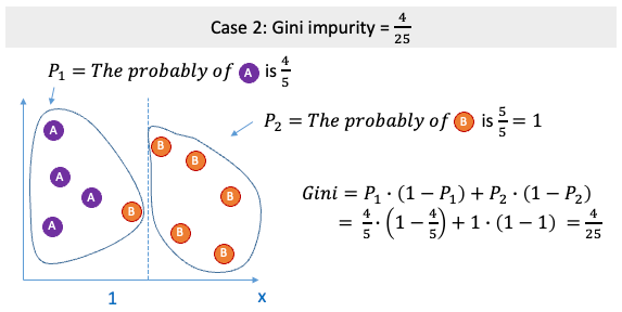
Q. What is the Gini Impurity in decision trees?
[Decision Trees] A decision tree model is a tree-like graph where sorting starts from the root node to the leaf node. It is built by using a heuristic called recursive partitioning. It splits the data into subsets, which then split repeatedly into even smaller subsets, and so on. It finds the variables that hold the most information about the target and then partitions the dataset along with the values of these variables. The process stops when the algorithm determines the data within the subsets are sufficiently pure. Here pure means homogeneity, i.e., if data can be separated accurately into classes and no data point is misclassified into another class (ideally!).
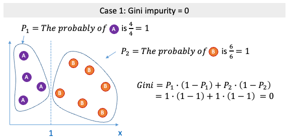
[Gini Impurity] The Gini impurity computes the likelihood that a randomly selected example would be incorrectly classified by a specific node. It ranges from 0 to 1, with 0 meaning the pure result. It is called an “impurity” value to indicate how data points are incorrectly classified.
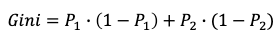
[Math Formula] Consider samples from two classes. The probability of samples belonging to Class 1 is P1 and Class 2 is (1-P2). The Gini impurity is:
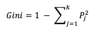
It can be extended to k classes. The probability of samples belonging to class j at a given node can be denoted as Pj. Then the Gini Impurity is defined as:
[Graph Representation for the Gini Impurity Calculation]
Q. How is variable importance determined in a random forest?
Credited to Leo Breiman in 1984, the variable importance in a random forest is the mean decrease in impurity (or gini importance). At each split in each tree, the decrease in impurity is the important measure for the splitting variable. For each variable, the random forest takes the average of the decrease in impurity across all trees.
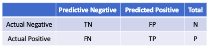
Q. What is a confusion matrix?
[What] A confusion matrix is a table to show how the predicted categories match the actual categories to measure the performance of a classification model. It reports the number of false positives, false negatives, true positives, and true negatives. (Click here to understand more.)
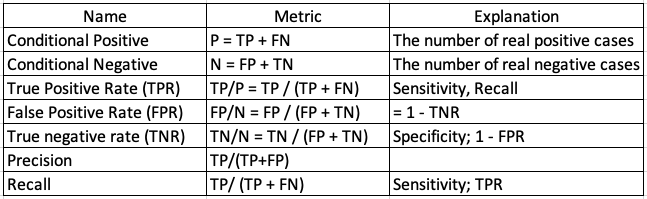
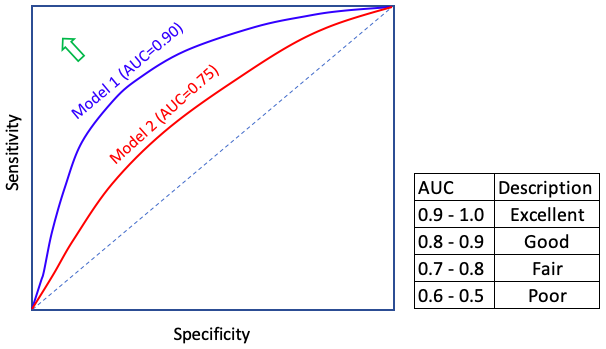
Q. What is the ROC curve?
[What] A confusion matrix evaluates a model given a certain threshold. But the threshold can vary from low to high. Is there a different measure that incorporates all ranges of the thresholds? Yes, the Receiver Operating Characteristic (ROC). It is an effective and popular evaluation metric because it visualizes the accuracy of predictions for a whole range of threshold values. The Receiver Operating Characteristic (ROC) curves plot TPR against FPR as shown below. The area under the ROC curve (AUC) assesses overall classification performance. The 4 dashed line means that you select the record by chance without any model guidance. If the ROC curve is on top of the dashed line, the AUC is 0.5 (half of the square area) and it means the model result is no different from a completely random draw. If the ROC curve is very close to the northwest corner, the AUC will be close to 1.0. The AUC is a value between 1.0 (excellent fit) to 0.5 (random draw). A rule-of-thumb is shown in the table. The predictability of a model can be considered “excellent” if the AUC is more than 0.9, and “good” if the AUC is above 0.8. (Click here to understand more.)
Q. Why is the ROC not an effective measure when the target is extremely imbalanced?
[What] The ROC curve is not sensitive enough if the target variable is extremely imbalanced. The AUC does not place more emphasis on one class over the other. The false positive rate (FPR) = FP/N. Because N is large and FP is small, the FPR will be small and insensitive to show changes in FP.
[So what] The Recall (PR) curves will be more informative than ROC when dealing with extremely imbalanced target data. Because Precision is directly influenced by class imbalance so the Precision-recall curves are better to highlight the differences between models for highly imbalanced data sets. The area under the Precision-Recall curve will be more sensitive than the area under the ROC curve. (Click here to understand more.)
Q. What is the bias-variance trade-off?
[What] The prediction error of a machine learning model is the gap between the actual and the predicted value that we try to minimize. This prediction error can be decomposed into two error terms: the bias term and the variance term. Image an archery (model) is shooting the target (actual) with multiple shots. Bias is how far the average of the shots away from the target (the bullseye); Variance is how close the multiple shots are to each other. If you want to reduce Bias, Variance will go up, and vice versa. there exists a trade-off between bias and variance.
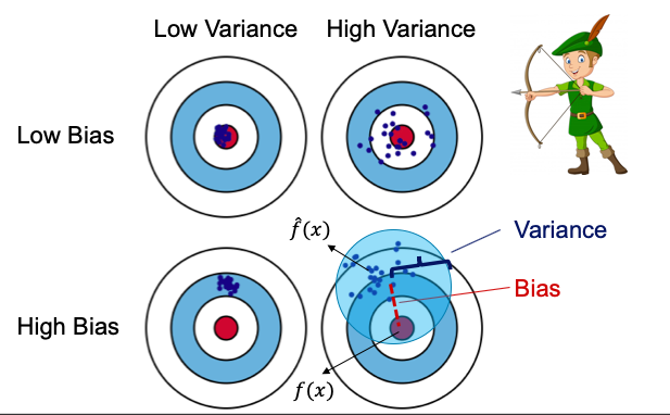
[So What] If we aim at reducing only one of the two, then the other will increase. Therefore we must aim at reducing both. There is a point where we can reduce both Bias and Variance without affecting the other and that point is what we are searching for. (Click here to understand more.)

Q. What is regularization and why is it useful?
[What] Regularization adds a penalty term to the loss function to penalize a large number of coefficients or a large magnitude of coefficients.
[So what] Overfitting does not just make your model inefficient, it could make the prediction very wrong. Suppose your final model has ten variables, eight of which capture the real patterns and the other two variables, noises. In other words, the two variables overfit noises and are useless. Suppose you are going to predict new data with your ten-variable model, and suppose the new values for the two variables are large. The prediction will be very wrong due to the two variables and the large values in the new data. So overfitting does not just make your model ineffective, it can make your prediction very wrong. That’s why we focus so much on attacking overfitting. (Click here to understand more.)
Q. Describe different regularization methods
[What]
- LASSO (Least Absolute Shrinkage and Selection Operator) — L1: It adds the sum of the absolute value of coefficients to the loss function. How do we remember “L1” or “L2”? A good way to remember “L1” is “1” which looks like the symbol for the absolute value.
- RIDGE — L2: It adds the sum of the squared value of coefficients to the loss function SSE. How do we remember “L2”? A good way to remember “L2” is the “2” in the “squared” terms in the equation.
- ElasticNet: is the combination of both L1 and L2. (Click here to understand more.)
Q. Why is LASSO used for feature selection?
[What] Jerome Friedman Trevor Hastie once said: ”Ridge regression is known to shrink the coefficients of correlated predictors towards each other, allowing them to borrow strength from each other.”
- In the extreme case of k identical predictors, the variables each get an identical coefficient with 1/kth. LASSO, on the other hand, tends to pick one and ignore the rest.
- Ridge reduces the magnitude of coefficients close to zero; in contrast, LASSO reduces the magnitude of coefficients exactly to zero. Therefore LASSO works like a feature selector that picks out the most important coefficients. (Click here to understand more.)
Q. How does an XGB control overfitting?
[What] The gradient boosting machine (GBM) algorithm does not have regularization so it is prone to overfitting. The XGBoosting (EXtreme Gradient Boosting) algorithm incorporates the regularization formalization in the loss function to control overfitting. (Click here to understand more.)
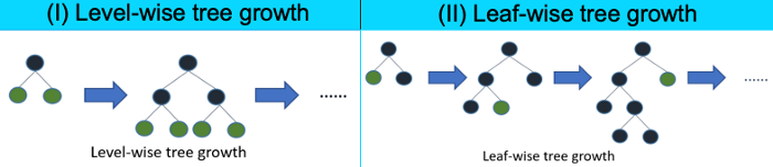
Q. Why is lightGBM prone to overfitting?
[What] LightGBM was developed to be a “fast, distributed, high-performance gradient boosting framework based on decision tree algorithms.
It uses the “leaf-wise” algorithm to achieve a higher level of accuracy as shown below. The leaf-wise tree grows on single branches to achieve precision. It could be very deep in a branch. In contrast, the level-wise tree tries to grow branches of the same level before moving to the next level. It looks more balanced. As the result, the leaf-wise tree growth is likely to over-fit when the data size is small. So you are advised to use parameter max_depth to limit the depth of tree <=3. (Click here to understand more.)
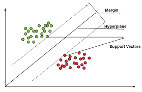
Q. Why does training an SVM takes a long time? How can I speed up?
[What] “Support Vector Machine” SVM is a supervised ML algorithm for regression or classification problems such as a binary target. It finds a hyperplane in N-dimensional space (N is the number of features) to classify the data points.
Many possible hyperplanes can separate the two classes of data points. We want to find the optimal hyperplane that can maximize the distance between data points of classes. This is called the maximum margin as shown in the following graph.
Since SVM calculates the distances for every data point, the computational time can be longer if the dataset is large.
[So What] You can take a fraction of random samples to reduce the computational time,
Q. Please mention at least three modeling techniques that can solve a multi-class classification problem.
[What] There are many algorithms for a multi-class problem.
- Multinomial/Multi-class Logistic Classification,
- Decision Tree,
- Random Forest,
- Naïve Bayes (NB),
- Gaussian Mixture Model (GMM),
- K-nearest Neighbors (KNN),
- Discriminant Analysis
- Support Vector Machine (SVM), and
- Neural Network (NN).
See my post “A Wide Variety of models for Multi-class Classification”.
Q. Which of the two neural network models is more complex?
- Model 1: 3 hidden layers with 300 neurons each.
- Model 2: 1 hidden layer with 500 neurons,
for a dataset that has 1 binary target variable, 150 numerical variables, and 50 categorical variables every 400 categories.
[What] The complexity of a model is shown in its number of parameters. Let’s compute the number of weightings for each model and compare. In general, you multiply the number of neurons in adjacent layers, then add up all the pairs. In this question, the categorical variables must be one-hot encoded to be a separate neuron.
- The 50 categorical will be transformed to 50 x 400 = 2,000 dummy variables. We have a total of 150 + 2,000 = 2,150 input neurons. The output has 1 neuron.
- Model 1: 2150 x 300 + 300 x 300 + 300 x 300 + 300 x 1 = 825,300
- Model 2: 2150 x 500 + 500 x 1 = 1,075,500
Model 2 has more parameters to be estimated so is more complex. (Click here to understand more.)
Q. If two predictors are highly correlated, what is the effect on the coefficients in the logistic regression? What are the confidence intervals of the coefficients? (Google)
[What] I will answer this question with a broad context. This question concerns multicollinearity. Multicollinearity is a common problem when estimating linear or generalized linear models (including logistic regression). When two independent variables are highly correlated, changes in one variable will associate with shifts in another variable. It becomes difficult for the model to estimate the relationship between each independent variable and the dependent variable separately, leading to unreliable and unstable estimates of regression coefficients.
The presence of multicollinearity causes individual p-values to be high and the confidence intervals to be wide. The confidence intervals may even include zero, which wrongly suggests a significant predictor be insignificant.
[So what]
A conventional view is if your goal is to predict the dependent variable Y accurately, multicollinearity is not a big issue. That view says your prediction will be accurate and the overall R-squared measures the goodness of fit. However, because the coefficients will be unstable and have large confidence intervals, the prediction accuracy will suffer. That being said, if your goal is to understand the relationship between a predictor and the dependent variable, multicollinearity is a big issue. The treatment is to apply regularization.
Q. What are the remedies for multicollinearity?
[What] You can consider the following techniques:
- Feature engineer the high-correlated variables into one variable. For example, the weight and height of a person are usually highly correlated. You can create a new variable “Body Mass Index”, which is a simple calculation of a person’s height and weight (Formula = weight (lb) / [height (in)]2 x 703).
- Increase sample size: this will make the confidence intervals of an estimate not as wide as before.
[Statistics & Probability]
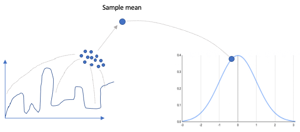
Q. Please describe the Central Limit Theorem.
[What] The central limit theorem (CLT) states that the sampling distribution of means will be approximately normal for large sample sizes (≥ 30), even if the original distribution is not normally distributed. The following figure explains CLT visually. Samples are taken from the original population with any shape of the distribution. The mean of the samples will become a point on a standard normal distribution. The standard deviation of this new normal distribution, called the standard error, will be the standard deviation of the original population divided by the square root of the sample size n.

Q. How do you derive the confidence interval from a series of coin tosses? (Google)
[What] Coin tossing follows the binomial distribution. Suppose there are N tosses, and the probability of head and tail is p and (1-p).
- Mean = p
- Variance = p(1-p)
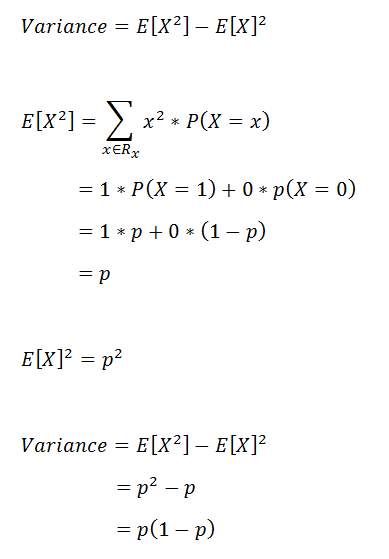
- Standard deviation =
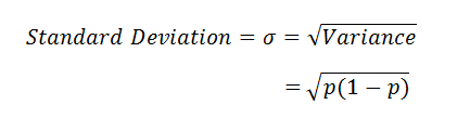
- Confidence Interval (C.I.) =
where z is the z score at 2.5% and 97.5%, approximately -1.96 and 1.96.
Q. What is the standard error of the mean? (Google)
[What] It is important to distinguish the followings:
- Population: Suppose a sample of N data points is drawn from a large population with a population mean u and unknown standard deviation.
- The sample mean & deviation: These N samples will have their sample mean x and its sample standard deviation s.
- Standard error of the mean: whenever samples are drawn from the population, the sample mean x will be around the true mean u. These sample means will follow a normal distribution with a standard deviation, called the standard error of the mean. It is the sample standard deviation divided by the square root of the sample size:

Q. What will happen if you simply duplicate the number of observations in linear regression?
[What] The duplications of the observations do not add any new information, so there will be no impact. Let’s examine the impact on each element, assuming a standard simple linear regression Y = X b + e.
- Correlation coefficient: no change. The formula below is the correlation coefficient.
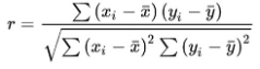
- R-squared: no change
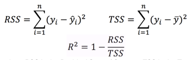

- Covariance between X and Y: no change. See the formula below. If n in the denominator is doubled, the summation in the nomination of cov(x,y) also will double, resulting in no change in the covariance.
- The variance of X: no change.
- Mean estimation of b: no change.
However, the following terms will change slightly:
- the standard error of b: all the point estimations of coefficient b will follow a standard normal distribution with the mean estimation of b and the standard error like the following red curve. The standard error is the sample deviation divided by the square root of the sample size. When the sample size doubles, the standard error will decrease. In other words, the standard normal distribution of b will become narrower like the blue curve.
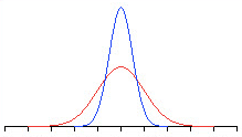
- t-stat for b: the t-stat is like a z score that measures the location between a point estimate and the mean, given the standard error SE. When the standard error SE becomes slightly smaller, the t-stat for b will increase slightly larger.

- p-value: t-stat and p-value go in the opposite direction. A small p-value is associated with a large t-stat. When the samples increase, the t-stat will increase and the p-value will decrease slightly. A p-value, or probability value, describes the probability that a point estimate b is zero. A p-value less than 0.05 (typically ≤ 0.05) is statistically significant. It indicates strong evidence against the null hypothesis, as there is less than a 5% probability the null is correct (and the results are random).
Q. What is the assumption of error in linear regression? (Google)
[What] The dependent variable Y doesn’t need to follow a normal distribution but the errors around a predicted Y should follow a normal distribution. The errors of a linear regression should follow a normal distribution, or the dependent variable has a conditional normal distribution. Data scientists often check the normality assumption from the histogram of the dependent variable. In this special case if the dependent variable follows a normal distribution, then the errors will be.
The four fundamental assumptions of linear regression are:
- The relationship between X and Y is linear
- Errors are normally distributed
- Homoskedasticity of errors (or, the equal variance around the line).
- Independence of the observations.
Q. What is the difference between K-means and the Gaussian mixture model (GMM)?
[What]
- K-means: Data usually do not uniformly distribute but cluster in data clusters. A popular technique to identify the clusters is the K-means clustering algorithm. This algorithm clusters data points to a fixed number of clusters. It computes the means, called the centroids, of each cluster and then calculates their distance to each of the data points. Each data point belongs to one and only one cluster. There is no probability such as a data point is 60% belonging to Cluster 1 and 40% to Cluster 2.
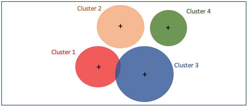
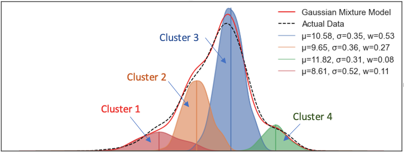
- GMM: The Gaussian mixture model delineates that the data come from k underlying clusters, each cluster follows a Gaussian distribution with a distinct mean and standard deviation. The graph below shows GMM models the contour of the data mix that come from 4 clusters with their means and standard deviations. A data point can belong to Cluster 1 with x1%, Cluster 2 with x2%, Cluster 3 with X3%, and Cluster 4 with x4%. All x1 to x4 should sum up to 1.0.
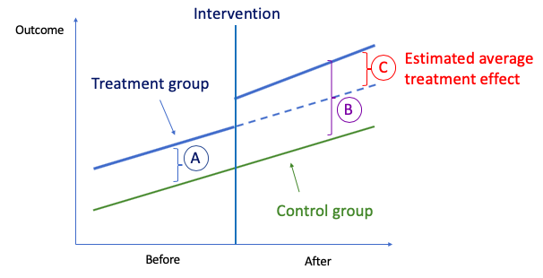
Q. Explain the basic maximum likelihood estimator (MLE). (Google)
[What]
- Maximum likelihood estimator: A good estimate of the unknown parameter θ would be the value of θ that maximizes the probability, or say the likelihood, of getting the data we observed. Suppose there are X1, …, Xn samples, the best value of θ will be the one that works for all X1, …, Xn values. This means the value of θ will result in the maximum probability of observing the data from the joint probability distribution, which is expressed below:
Q. What is the difference between the maximum likelihood estimation (MLE) and the expectation-maximization (EM) algorithm? (Google)
[What]
- Maximum likelihood estimation (MLE) finds the best parameter value that maximizes the probability that the data comes from.
- The expectation-maximization algorithm is similar to MLE in the presence of latent variables. It first estimates the values of the latent variables, then optimizes the model.
[So what]
- EM is commonly used in the Gaussian Mixture Model.
Q. How could you do an A/B test if we see a 3% increase for the product? (Google)
[What]
A/B testing is a way to compare two versions of something to determine which performs better. For example, a team wants to test two versions of a website, the current layout and the new layout, to see which layout results in a higher rate of purchasing items. The current layout is the A version — the control group, and the new one the B version — the treatment group. It is a randomized experimental test.
- Null & alternative hypotheses: the null hypothesis is the one that there is no difference between the control A and the treatment B group. The alternative hypothesis says there is a statistically significant difference between the two groups.
- Testing metric: this is the goal that you want to change. In our case, it is the rate of purchase.
- Randomly assign visitors to each version so ideally, the only difference is the layout. We know in real life there are many other factors affecting the purchase decision of a customer. The randomization tries to minimize the chances that other factors drive the testing results.
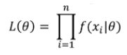
Q. To find the causal relationship between the two measures, we may set up a randomized control trial (RCT) to identify. But suppose an RCT is infeasible, what can we do?
[What] One technique that can help to identify the causal relationship between two variables is the Difference-in-Differences (DiD) technique.
The idea behind DiD is simple. First, we compute the difference in the mean of the outcome between the two groups in the “Before” period, and we compute the same for the “After” period. Then we take the “second difference”, which is the difference between the means in the before period and the after period. This second difference measures how the change in outcome differs between the two groups. The difference is attributed to the causal effect of the intervention. (Click here to understand more.)
Q7. What is the difference between parametric and non-parametric testing?
[What]
- Parametric tests: assume the data come from underlying statistical distributions. For example, Student’s t-test is typically used for two independent samples. But the t-test is only valid if each sample follows a normal distribution
- Nonparametric tests: do not rely on any distribution. They can thus be applied even if parametric conditions of validity are not met. So it is more robust than parametric tests.
[So what]
In a test that compares the means between two distinctly independent groups, the parametric test procedure is typically a two-sample t-test, and the non-parametric test is the Wilcoxon rank sum test.
Summary
Many of these questions and answers are drawn from dataman’s articles. You can dig deeper into the following articles:


