
Revisiting the ROC and the Precision-Recall Curves
I have written a series of articles on the techniques for machine learning modeling with extremely imbalanced target data, and in such cases, the ROC curve is not a sensitive measure. However, I believe it will be helpful to showcase a model prediction example. In this article, I will show you
- How to construct the ROC curve from the confusion matrix,
- Why the ROC curve is not sensitive enough when the target is extremely imbalanced, and
- How to read a Precision-recall Curve.
I also build the Python code snippets for those of you who may be interested.
(1) What Is Imbalanced Data?
The definition of imbalanced data is straightforward. A dataset is imbalanced if at least one of the classes of the target variable constitutes only a very small minority. In a supervised machine learning model, the class imbalance in the target variable can result in a serious bias towards the majority class and reduce the predictability. Imbalanced data prevail in banking, insurance, engineering, and many other fields. It is common in fraud detection that the imbalance is on the order of 100 to 1.
(2) Let’s Start with the Confusion Matrix
Assume the target variable is binary and you build a binary model called a binary classifier. Your model prediction for each record will be a continuous probability from 0.0 to 1.0. You will decide on a cutoff to label the predictions as Positive/Negative Yes/No or 1/0.
The performance of a model can be represented in a confusion matrix with four categories. Let’s use the labels “positive” or “negative” for either Positive/Negative or Yes/No or 1/0. True positives (TP) are positive examples that are correctly labeled as positives, and False positives (FP) are negative examples that are labeled incorrectly as positive. Likewise, True negatives (TN) are negatives labeled correctly as negative, and false negatives (FN) refer to positive examples labeled incorrectly as negative. A good model is expected to have more true positives and fewer false positives.
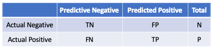
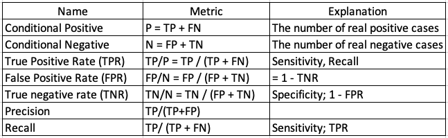
Given the above confusion matrix, we can define the following:
(3) The ROC curve
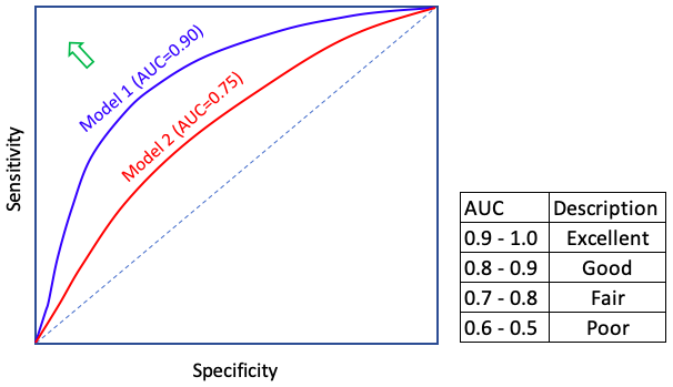
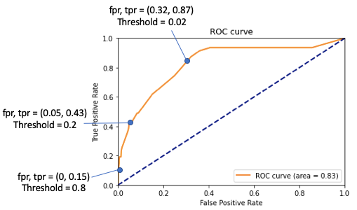
A confusion matrix evaluates a model given a certain threshold. But the threshold can vary from low to high. Is there a different measure that incorporates all ranges of the thresholds? Yes, the Receiver Operating Characteristic (ROC). It is an effective and popular evaluation metric because it visualizes the accuracy of predictions for a whole range of threshold values. The Receiver Operating Characteristic (ROC) curves plot TPR against FPR as shown below. The area under the ROC curve (AUC) assesses overall classification performance. The 4 dashed line means you select the record by chance without any model guidance. If the ROC curve is on top of the dashed line, the AUC is 0.5 (half of the square area) and it means the model result is no different from a completely random draw. If the ROC curve is very close to the northwest corner, the AUC will be close to 1.0. The AUC is a value between 1.0 (excellent fit) to 0.5 (random draw). A rule-of-thumb is shown in the table. The predictability of a model can be considered “excellent” if the AUC is more than 0.9, and “good” if the AUC is above 0.8.
(4) The ROC Is Not Sensitive If the Target Is Extremely Imbalanced
However, the ROC curve is not sensitive enough if the target variable is extremely imbalanced. The AUC does not place more emphasis on one class over the other, so it does not reflect the minority class well. The false positive rate (FPR) = FP/N. Because N is large and FP is small, the FPR will be small and insensitive to show changes in FP.
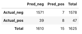
Let’s use the above number example with an imbalanced target to understand this. The actual positives (P) in this example are only 47 out of the total 1625.
- TPR (TP/P) = 8/47 = 0.17.
- FPR (FP/N) = 7/1578 = 0.004. It somehow reflects the size of the majority but is not direct.
- Precision TP/(TP+FP) = 8/(8+7) = 0.53
- Recall TP/(TP+FN) = 8/(8+39) = 0.17
Do you notice the denominator is not N but FN? We know false negatives (FN) are positive cases labeled incorrectly as negative. If a model mislabels all positives as negatives, the FN will be large and FPR will be small.
(5) The Precision-Recall (PR) Curve
Davis and Goadrich in this paper propose that Precision-Recall (PR) curves will be more informative than ROC when dealing with highly skewed datasets. The PR curves plot precision vs. recall (FPR). Because Precision is directly influenced by class imbalance so the Precision-recall curves are better to highlight the differences between models for highly imbalanced data sets. When you compare different models with imbalanced settings, the area under the Precision-Recall curve will be more sensitive than the area under the ROC curve.
Is there a way to compute the Area under Precision-Recall Curve as the AUC under the ROC curve? The short answer is the Average Precision (AP). The AP summarizes a precision-recall curve as the weighted mean of precisions achieved at each threshold. See the formula here. Because Precision and Recall are always between 0 and 1, AP falls within 0 (very poor) and 1 (excellent fit) also.
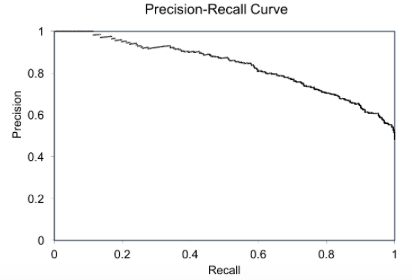
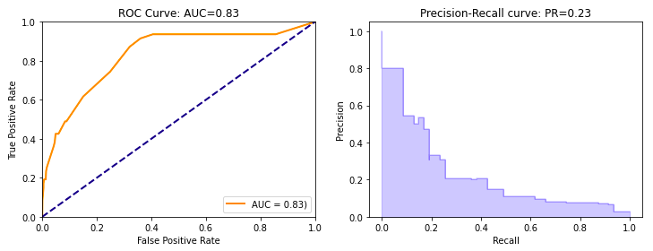
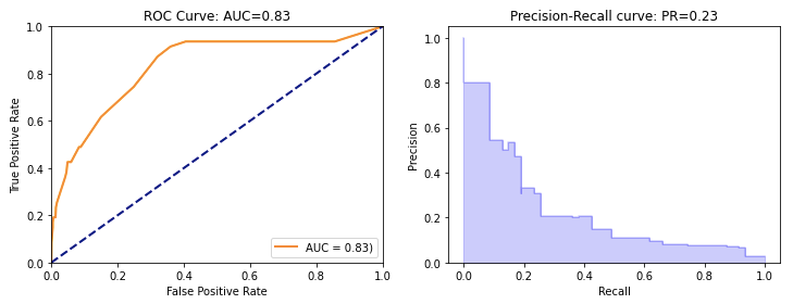
In the code example below, I will build a model for an extremely imbalanced target. The model is poor but the ROC still shows 0.83. In contrast, the Area Under the PR curve is 0.26 which is much less than 1.0.
(6) Build a Model for an Extremely Imbalanced Target
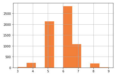
I am going to use the wine quality data in Kaggle.com to create an extremely imbalanced binary target. The target value of this dataset is the quality rating from low to high (0–10) as shown below. To make the target extremely imbalanced, I define those ≥ 8.0 to be “1” and the rest to be “0”. This results in a very imbalanced target (3% “1”s and 97% “0”s). The notebook is available via this link.
Because the purpose of this article is to illustrate the CM, ROC, and PR and not the model itself, I just build a very simple decision tree model. The variance importance chart is available in the notebook.
The DecisionTreeClassier in Scikit-learn has two prediction functions.
.predict(): This returns a binary outcome 0 and 1. The cutpoint of predict() is 0.50. The above sample code uses this function..predict_prob(): This returns the probability of 0 and 1 in [p0, p1]. We are interested in the probability of 1 so we will choose p1 below.
(7) A Confusion Matrix Corresponds to a Point on the ROC Curve
As explained earlier, the ROC curve is derived from the confusion matrix with varying thresholds. A confusion matrix corresponds to a point on a ROC curve. The scikit-learn function roc_curve() does this job. But instead of using the canned function, I also want to show you how to construct the ROC curve manually so you will see the relationships between the confusion matrix and the ROC curve.
(7.1) Construct the ROC curve manually
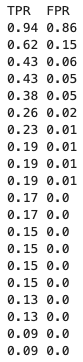
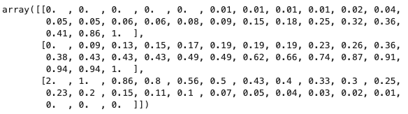
The following code snippet takes the actual Y, the predicted Y, and a given threshold to construct the confusion matrix, the True Positive Rate, and the False Positive Rate. I mimic the definitions in Figures I and II so you can compare.

By varying a range of the thresholds, I can produce the corresponding confusion matrices, the true positive rates, and the false positive rates. With these statistics, I make the ROC curve.
(7.2) Automate the ROC Curve with the Scikit-learn roc_curve()
(8) The PR Curve Measures Better for the Extremely Imbalanced Case
The following code snippet puts the ROC curve and the Precision-Recall (PR) curves side-by-side. Here we see the ROC is still as high as 0.83 and the PR is only 0.23<<1.0. The PR reflects the true quality of the model performance.
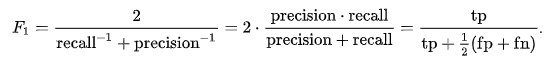
(9) The F1 Score Is Another Good Measure
The F1 score can be interpreted as a weighted average of the precision and recall, where an F1 score reaches its best value at 1 and worst score at 0. It is the harmonic mean of precision and recall, meaning the relative contribution of precision and recall to the F1 score are equal:
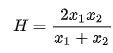
The harmonic mean has wide applications in physics, finance, and geometry and is expressed as the following:
Below we use F1 to measure our model performance. It is 0.26<<1.0, so the model has room to improve. The under-sampling or over-sampling techniques can be used to improve the model performance. Note that an aggressive over-sampling or under-sampling may not yield a large increase in the model performance.
(10) Use Under-sampling or Over-sampling Techniques
The issue of class imbalance can result in a serious bias towards the majority class, reducing the classification performance and increasing the number of false negatives. How can we alleviate the issue? The most commonly used techniques are data resampling either under-sampling the majority of the class, over-sampling the minority class, or a mix of both. I summarized the techniques to address the issue of imbalanced data in the previous articles “Using Under-Sampling Techniques for Extremely Imbalanced Data” and “Using Over-Sampling Techniques for Extremely Imbalanced Data”.
Conclusion
I hope this article gives you a better understanding of this topic. I have made the code in this article available for download via this link. If you like to have a comprehensive review, the following sequence will help:


