Using Under-Sampling Techniques for Extremely Imbalanced Data

The issue of class imbalance can result in a serious bias towards the majority class, reducing the classification performance and increasing the number of false negatives. How can we alleviate the issue? The most commonly used techniques are data resampling either under-sampling the majority of the class, or oversampling the minority class, or a mix of both. This will result in improved classification performance. In this article, I will explain what is imbalanced data, why ROC fails to measure correctly, and the techniques to attack the issue. You are highly recommended to read the second article “Using Over-Sampling Techniques for Extremely Imbalanced Data”. In both articles, I include the Python code for those who are interested. To access the code in Python Notebook, you can click here.

What is imbalanced data?

The definition of imbalanced data is straightforward. A dataset is imbalanced if at least one of the classes constitutes only a very small minority. Imbalanced data prevail in banking, insurance, engineering, and many other fields. It is common in fraud detection that the imbalance is on the order of 100 to 1.

Why a ROC curve cannot measure well?

The Receiver operating characteristic (ROC) curve is the typical tool for assessing the performance of machine learning algorithms, but it does not measure well for imbalanced data.

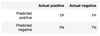
Let’s formulate this decision problem with the labels as either positive or negative. The performance of a model can be represented in a confusion matrix with four categories. True positives (TP) are positive examples that are correctly labeled as positives, and False positives (FP) are negative examples that are labeled incorrectly as positive. Likewise, True negatives (TN) are negatives labeled correctly as negative, and false negatives (FN) refer to positive examples labeled incorrectly as negative.

Given the confusion matrix, we can define the matrix:

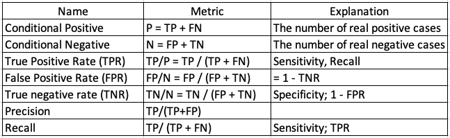
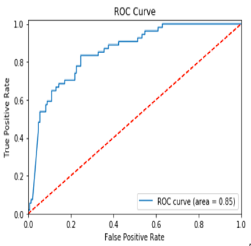
The above table shows TPR is TP / P, which depends only on positive cases. The Receiver Operating Characteristic (ROC) curves plot TPR against FPR, as shown below. The area under the ROC curve (AUC) assesses overall classification performance. AUC does not place more emphasis on one class over the other, so it does not reflect the minority class well. Remember that the red dashed line in Figure A is the result when there is no model and the data are randomly drawn. The blue curve is the ROC curve. If the ROC curve is on top of the red dashed line, the AUC is 0.5 (half of the square area) and it means the model result is no different from a completely random draw. On the other hand, if the ROC curve is very close to the northwest corner, the AUC will be close to 1.0. So the AUC is a value between 1.0 (excellent fit) to 0.5 (random draw).

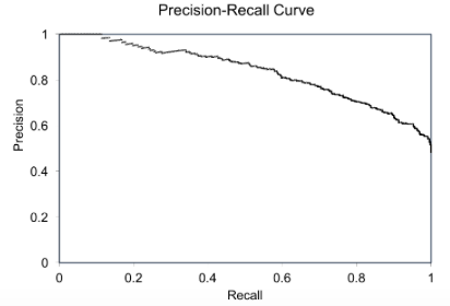
Davis and Goadrich in this paper propose that Precision-Recall (PR) curves will be more informative than ROC when dealing with highly skewed datasets. The PR curves plot precision vs. recall (FPR). Because Precision is directly influenced by class imbalance so the Precision-recall curves are better to highlight differences between models for highly imbalanced data sets. When you compare different models with imbalanced settings, the area under the Precision-Recall curve will be more sensitive than the area under the ROC curve.

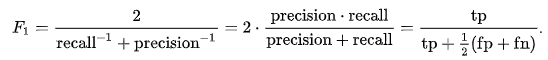
The F1 Score

The F1 score should be mentioned here. It is the harmonic mean of precision and recall as the following:

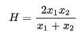
The harmonic mean has wide applications in physics, finance, and geometry and is expressed as the following:

What are the remedies?

Broadly speaking there are three major approaches to handling imbalanced data: data sampling, algorithm modifications, and cost-sensitive learning. In this chapter, I will focus on the data sampling techniques.

Using undersampling techniques

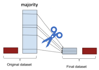
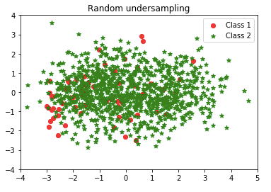
(1) Random under-sampling for the majority class

A simple under-sampling technique is to under-sample the majority class randomly and uniformly. This can potentially lead to the loss of information. But if the examples of the majority class are near to others, this method might yield good results.

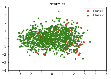
(2) NearMiss

To attack the issue of potential information loss, the “near neighbor” method and its variations have been proposed. The basic algorithms of the near neighbor family are this: first, the method calculates the distances between all instances of the majority class and the instances of the minority class. Then k instances of the majority class that have the smallest distances to those in the minority class are selected. If there are n instances in the minority class, the “nearest” method will result in k*n instances of the majority class.

“NearMiss-1” selects samples of the majority class their average distances to the three closest instances of the minority class are the smallest. “NearMiss-2” uses three farthest samples of the minority class. “NearMiss-3” selects a given number of the closest samples of the majority class for each sample of the minority class.

(3) Condensed Nearest Neighbor Rule (CNN)

To avoid losing potentially useful data, some heuristic undersampling methods have been proposed to remove redundant instances that should not affect the classification accuracy of the training set. Hart (1968) introduced the Condensed Nearest Neighbor Rule (CNN). Hart starts with two blank datasets A and B. Initially the first sample is placed in dataset A, while the rest samples are placed in dataset B. Then one instance from dataset B is scanned by using dataset A as the training set. If a point in B is misclassified, it is transferred from B to A. This process repeats until no points are transferred from B to A.

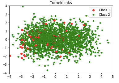
(4) TomekLinks

In the same manner, Tomek (1976) proposed an effective method that considers samples near the borderline. Given two instances a and b belonging to different classes and are separated by a distance d(a,b), the pair (a, b) is called a Tomek link if there is no instance c such that d(a,c) < d(a,b) or d(b,c) < d(a,b). Instances participating in Tomek links are either borderline or noise so both are removed.

(5) Edited Nearest Neighbor Rule (ENN)

Wilson (1972) introduced the Edited Nearest Neighbor Rule (ENN) to remove any instance whose class label is different from the class of at least two of its three nearest neighbors. The idea behind this technique is to remove the instances from the majority class that is near or around the borderline of different classes based on the concept of nearest neighbor (NN) to increase the classification accuracy of minority instances rather than majority instances.

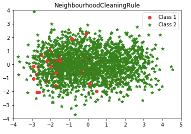
(6) NeighbourhoodCleaningRule

The neighborhood Cleaning Rule (NCL) deals with the majority and minority samples separately when sampling the data sets. NCL uses ENN to remove the majority of examples. for each instance in the training set, it finds three nearest neighbors. If the instance belongs to the majority class and the classification given by its three nearest neighbors is the opposite of the class of the chosen instance, then the chosen instance is removed. If the chosen instance belongs to the minority class and is misclassified by its three nearest neighbors, then the nearest neighbors that belong to the majority class are removed.

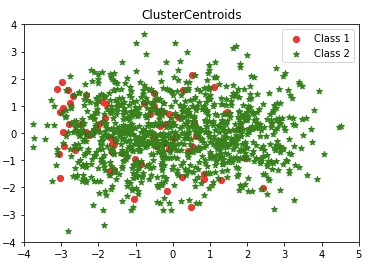
(7) ClusterCentroids

This method undersamples the majority class by replacing a cluster of majority samples This method finds the clusters of the majority class with K-mean algorithms. Then it keeps the cluster centroids of the N clusters as the new majority samples.

Python code

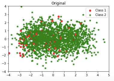
Below I demonstrate the sampling techniques with the Python scikit-learn module imbalanced-learn. The notebook is available via this Github link. Readers need to install the Python package using pip or conda install. The following data generation progress (DGP) generates 2,000 samples with 2 classes. The data is extremely unbalanced with the proportion of 0.03 and 0.97 assigned to each class. There are 10 features, of which 2 are informative and 2 are redundant and 6 (10–2–2) are repeated features. The make_classification function generates the repeated (useless) features from the informative and redundant features. The redundant features are simply the linear combinations of informative features. Each class has consisted of 2 gaussian clusters. For each cluster, informative features are drawn independently from N(0, 1) and then linearly combined within each cluster. It is important to know if the parameter weights are left blank, then classes are balanced.

It is also important to note that you only do under-sampling or over-sampling on the training data, leaving the test data untouched. In another word, you do not apply the under-sampling/over-sampling to your test data. You shall build the model on your under-sampled/over-sampled training data, and validate your model on your untouched test data.

For ease of visualization, I use principal component analysis to reduce the dimensions and pick the first two principal components. A scatterplot for the dataset is shown below.

Isn’t it interesting? How about the over-sampling techniques? The second article “Using Over-Sampling Techniques for Extremely Imbalanced Data” shows you more!

Additional Note when Applying in H2O

For data scientists who use H2O.ai, how do you apply the above sampling techniques? If you are not familiar with H2O, the post “My Lecture Notes on Random Forest, Gradient Boosting, Regularization, and H2O.ai” shows the H2O code snippets for various algorithms.

It is fairly easy to do so. From the above sampling code snippets, you get the sampled data X_rs and the corresponding y labels y_rs. All you need to do is to concatenate X_rs and y_rs to a data frame, then convert to an H2O data frame as usual.

This chapter is part of the book series “Handbook of Anomaly Detection with Python Outlier Detection.” For easy navigation to chapters, I list the chapters at the end.

• Chapter 1 — Introduction
• Chapter 2 — Histogram-Based Outlier Score (HBOS)
• Chapter 3 — Empirical Cumulative Outlier Detection (ECOD)
• Chapter 4 — Isolation Forest (IForest)
• Chapter 5 — Principal Component Analysis (PCA)
• Chapter 6 — One-Class Support Vector Machine (OCSVM)
• Chapter 7 — Gaussian Mixed Models (GMM)
• Chapter 8 — K-nearest Neighbors (KNN)
• Chapter 9 — Local Outlier Factor (LOF)
• Chapter 10 — Clustering-Based Local Outlier Factor (CBLOF)
• Chapter 11 — Extreme Boosting-Based Outlier Detection (XGBOD)
• Chapter 12 — Autoencoders
• Chapter 13 — Under-sampling for Extremely Imbalanced Data
• Chapter 14 — Over-sampling for Extremely Imbalanced Data

Readers are recommended to purchase books by Chris Kuo:

• The explainable AI: https://a.co/d/cNL8Hu4
• Transfer learning for image classification: https://a.co/d/hLdCkMH
• Modern time series anomaly detection: https://a.co/d/ieIbAxM
• Handbook of Anomaly Detection: https://a.co/d/5sKS8bI