Handbook of Anomaly Detection: with Python Outlier Detection — (2) HBOS

Consider multi-dimensional data like a data frame in an Excel Spreadsheet. The columns are the dimensions or variables, and the rows are the observations. An observation had multiple values. The count statistic of a variable is called the histogram. If there are N variables, there will be N histograms. If a value of observation falls in the tail of a histogram, the value is an outlier. If many values of observation are outliers, the observation is very likely to be an outlier.

The columns are also called variables. With all the observations, we can derive the count statistic, called a histogram, for each variable. If a value of observation falls in the tail of a histogram, the value is an outlier. It is often the case that some values of observation are outliers in terms of the corresponding variables, but some values are normal. If many values of observation are outliers, the observation is very likely to be an outlier.

With this intuition, the histogram of a variable can be used to define the univariate outlier score for a variable. An observation shall have N univariate outlier scores. The technique assumes independence between variables to derive histograms and the univariate outlier scores. The N univariate outlier scores of an observation can be summed up to become the Histogram-based Outlier Score (HBOS). Although this assumption may sound strong, HBOS proves its effectiveness in real-world cases.

(A) How Does the HBOS Work?

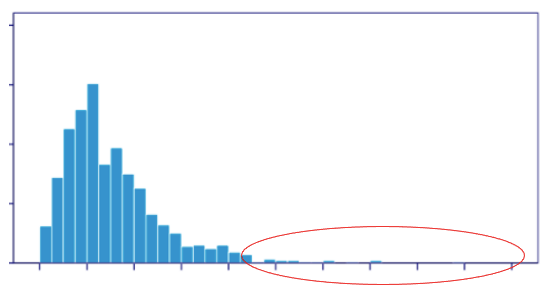
The HBOS constructs the histograms independently for all the N variables. The height of the bin is used to measure the “outlier-ness”. Most of the observations belong to the bins of high frequency, and outliers belong to the bins of low frequency. The univariate outlier score is defined as the inverse of the height of a bin.

The HBOS is formally defined as the sum of the logarithmic univariate outlier score of the N variables:

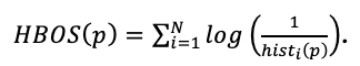
In the above equation, hist_i(p) is the height of the bin of variable i where Observation p belongs to, and 1/hist(p) is the univariate outlier score. This definition will associate a large value to an outlier.

If a variable is categorical, the histogram is the count by category. If a variable is numeric, it shall first be discretized into bins of equal width to derive the count statistic. The maximum height of each histogram is normalized to 1.0. This ensures all the univariate scores can be summed up equally to get the HBOS.

(B) Distribution-Based Algorithms Can Be Fast

In the previous chapter, I mentioned anomaly detection algorithms can be proximity-based, distribution-based, or ensemble-based methods. Distribution-based methods fit data with probability distributions to get outlier scores. The computational time of distribution-based methods is generally shorter than the time of the proximity-based or the ensemble-based methods. A proximity-based method can be time-consuming because it needs to compute the distance between any two data points. For this reason, it is a good modeling candidate for a data science project to start with.

(C) Modeling Procedure

In this book, I apply the procedure in Figure (C) that helps you to develop the model, assess the model performance, and demonstrate the model outcome. They are (1) Model development, (2) Threshold determination, and (3) Profile the normal and abnormal groups.

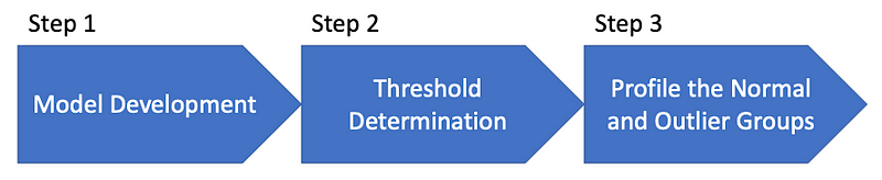
In most cases we do not have the verified outliers to conduct supervised learning modeling. Since we do not have the known outliers, we do not even know the percentage of outliers in a population. The good news is the outlier scores already measure the deviation of an observation from the normal data. If we derive the histogram for the outlier scores, we can discover those observations and determine the percentage of the outliers. Therefore, In Step 1 we develop the model and assign outlier scores. In Step 2, we plot the outlier scores in a histogram, then choose a value, called the threshold, to separate normal observations from abnormal observations. The threshold also determines the size of the abnormal group.

How do we assess the soundness of an unsupervised model? If a model can effectively identify outliers in the training data, those outliers should show the characteristics of outlier-ness. They should be very different from the normal data in terms of those variables. In Step 3, we will profile the normal and outlier groups to prove the soundness of the model. The descriptive statistics (such as the means and standard deviations) of the variables between the two groups prove the model predictability.

The descriptive statistic table is a reasonable metric to evaluate whether a model is consistent with any prior knowledge. If a variable is expected to be higher or lower in the outlier group but the result is counter-intuitive, you shall investigate, modify, or drop the variable and do modeling again. The final version of a model should deliver a descriptive statistic table that is consistent with any prior knowledge.

(C.1) Step 1 — Build your Model

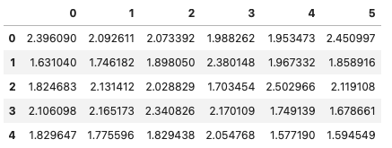
Like before, I will use the utility function generate_data() of PyOD to generate ten percent outliers. To make the case more interesting, the data generation process (DGP) will create six variables. Although this mock dataset has the target variable Y, the unsupervised models only use the X variables. The Y variable is simply for validation. I set the percentage of outliers to 5% with “contamination=0.05.”

The first five records look like the following:

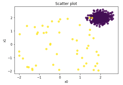
Let me plot the first two variables in a scatter plot. The yellow points are the outliers and the purple points are the normal data points.

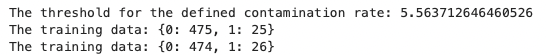
Let’s build our first HBOS model. An important hyper-parameter for HBOS is the number of bins. HBOS can be sensitive to the bin width of the histogram, and we will discuss this hyper-parameter later. This model assumes the number of bins to be 50. In this model we also assume the contamination rate to be 5% because we have generated 5% outliers in the data. If we do not specify it, the default is 10%.

Once trained, the model also realizes the outlier scores for the observations in the training data. If we sort the observations in ascending order, those observations higher than the threshold are outliers. This threshold is determined by the parameter contamination=0.05, which means 5% of the data will be outliers. The model calculates the threshold of the training data and stores in HBOS.threshold_.

We will use the function decision_function() of PyOD to produce the outlier scores for the training and test data. We will also use the function predict() to predict where an observation is an outlier or not. The function predict() compares the the outlier scores with the thresholdhbos.threshold_. If an outlier score is higher than the threshold, the function assigns “1” to an observation and otherwise “0”. I made a short function count_stat() to show the count of predicted “1” and “0” values.

(C.2) Step 2 — Determine a reasonable threshold

In most cases, we do not know the percentage of outliers. How can we identify outliers in an unsupervised learning model? Because the outlier score already measures the deviation of a data point from others, we can sort the data by their outlier scores. Those data points with high outlier scores can be outliers. We can determine a threshold based on the outlier scores to separate outliers from normal data.

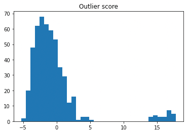
Figure (C.2) presents the histogram of outlier score. We may choose a more conservative approach by selecting a high threshold, which will result in fewer but hopefully finer outliers in the outlier group. The histogram suggests 5.5 to be the threshold. The selection of the threshold also determines the percentage of outliers in the population.

(C.3) Step 3 — Present the summary statistics of the normal and the abnormal groups

This step profiles the characteristics of the normal and abnormal groups. The characteristics of the outliers should be very different from the normal data. The descriptive statistic table becomes a good metric to prove the soundness of a model.

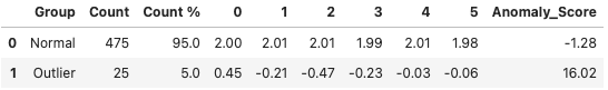
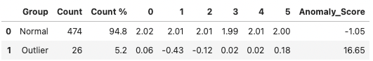
In Table (A) I show the count and count percentage of the normal and outlier groups. In our case there are two features labeled as “Feature 0” and “Feature “1”. The “Anomalous_Score” is the average anomaly score. You are reminded to label the features with their feature names for an effective presentation. The table tells us several important results:

• The size of the outlier group: The outlier group is about 8.4%. Remember the size of the outlier group is determined by the threshold. If you choose a higher value for the threshold, the size will shrink.
• The average anomaly score: The average HBO score of the outlier group is far higher than that of the normal group (5.836 > -0.215). This evidence just verifies the data in the outlier group are outliers. At this point, you do not need to interpret too much on the scores.
• The feature statistics in each group: Table (A) shows the outlier group has smaller values for Feature ‘0’ and Feature ‘1’ than those of the normal group. In a business application, you probably expect that the feature values in the outlier group should be higher or lower than those of the normal group. Therefore the feature statistics help to make sense of the model results.

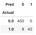
Since we have the ground truth y_test in our data generation, we can produce a confusion matrix to understand the model performance. The data generation process produced 50 outliers (500 x 10% = 50). The model delivers a decent job and identifies 42 out of 50 with a threshold of 4.0.

(D) Achieve Model Stability by Aggregating Multiple Models

HBOS can be sensitive to the bin width of the histogram. If the bins are too narrow, the normal data points falling in these bins will be identified as outliers. If the bins are too wide, outliers will fall into the bins of the normal data and be overlooked. To produce a model with a stable outcome, the strategy is to build HBOS models with a range of histogram widths to obtain multiple scores and then aggregate the scores. This approach will reduce the chance of overfitting and increase prediction accuracy. The PyOD module offers four methods to aggregate the outcome. You only need to use one method to produce your aggregate outcome.

1. Average
2. Maximum of Maximum (MOM)
3. Average of Maximum (AOM)
4. Maximum of Average (MOA)

I am going to produce 10 HBOS models for a range of bins [5,10, 15, 20, 35, 30, 50, 60, 75, 100]. The average prediction of these models will be the final model prediction.

from pyod.models.combination import aom, moa, average, maximization
from pyod.utils.utility import standardizer
from pyod.models.hbos import HBOS

# Standardize data
X_train_norm, X_test_norm = standardizer(X_train, X_test)

# Test a range of binning 
k_list = [5, 10, 15, 20, 25, 30, 50, 60, 75, 100]
n_clf = len(k_list)
# Just prepare data frames so we can store the model results
train_scores = np.zeros([X_train.shape[0], n_clf])
test_scores = np.zeros([X_test.shape[0], n_clf])

# Modeling
for i in range(n_clf):
    k = k_list[i]
    hbos = HBOS(n_bins=k)
    hbos.fit(X_train_norm)
    # Store the results in each column:
    train_scores[:, i] = hbos.decision_function(X_train_norm) 
    test_scores[:, i] = hbos.decision_function(X_test_norm) 
# Decision scores have to be normalized before combination
train_scores_norm, test_scores_norm = standardizer(train_scores,test_scores)

The ten outlier scores are stored in the above “train_scores”. The normalization step is needed for the ten scores in order to aggregate them correctly. The average predictions of the 10 scores is in “y_by_average” below. I create its histogram in Figure (D).

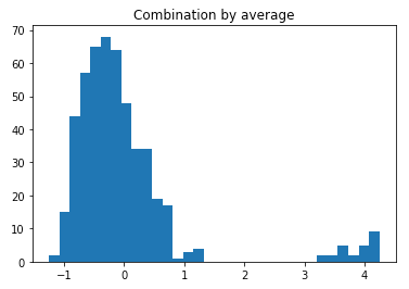
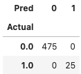
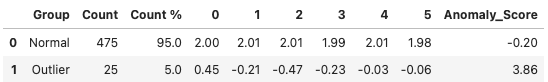
The histogram in Figure (D) suggests a threshold of 1.4. The descriptive statistics with this threshold are shown in Table (D). It identifies 25 data points to be the outliers. Readers shall apply similar interpretations to Table (C.3).

(E) Summary of the HBOS Algorithm

• If an observation is an outlier in terms of almost all variables, the observation is likely an outlier.
• The HBOS defines the outlier score for each variable based on its histogram.
• The outlier scores of all variables can be added up to get the multivariate outlier score for an observation.
• Because histograms are easy to construct, the HBOS is an efficient unsupervised method to detect anomalies.

(F) Python Notebook: Click here for the notebook.

References

• [1] Goldstein, M., & Dengel, A. (2012). Histogram-based outlier score (HBOS): A fast unsupervised anomaly detection algorithm. KI-2012: poster and demo track, 9.

For easy navigation to chapters, I list the chapters at the end.

• Chapter 1 — Introduction
• Chapter 2 — Histogram-Based Outlier Score (HBOS)
• Chapter 3 — Empirical Cumulative Outlier Detection (ECOD)
• Chapter 4 — Isolation Forest (IForest)
• Chapter 5 — Principal Component Analysis (PCA)
• Chapter 6 — One-Class Support Vector Machine (OCSVM)
• Chapter 7 — Gaussian Mixed Models (GMM)
• Chapter 8 — K-nearest Neighbors (KNN)
• Chapter 9 — Local Outlier Factor (LOF)
• Chapter 10 — Clustering-Based Local Outlier Factor (CBLOF)
• Chapter 11 — Extreme Boosting-Based Outlier Detection (XGBOD)
• Chapter 12 — Autoencoders
• Chapter 13 — Under-sampling for Extremely Imbalanced Data
• Chapter 14 — Over-sampling for Extremely Imbalanced Data

Readers are recommended to purchase books by Chris Kuo:

• The explainable AI: https://a.co/d/cNL8Hu4
• Transfer learning for image classification: https://a.co/d/hLdCkMH
• Modern time series anomaly detection: https://a.co/d/ieIbAxM
• Handbook of Anomaly Detection: https://a.co/d/5sKS8bI