
Handbook of Anomaly Detection: With Python Outlier Detection — (8) KNN

(Revised on December 9, 2022)
The K-nearest neighbor algorithm, known as KNN or k-NN, probably is one of the most popular algorithms in machine learning. KNNs are typically used as a supervised learning technique where the target labels are provided. KNNs can also be used for the computation of the distance to the k neighbors. Because the latter does not use a target variable, some on-line sources such as the scikit-learn KNN [1] calls it unsupervised learning. The KNN in PyOD uses the latter. It computes the distance to the k neighbors and uses the distance to define the outlier scores.
In the beginning of the chapter, I will dedicate some space to clarify how KNN can be used in a supervised learning or unsupervised learning. Then I will explain how KNN defines the outlier score for anomaly detection.
(A) Use KNN as Unsupervised Learning Technique
The unsupervised k-NN method computes the Euclidean distance of observation to other observations. The unsupervised KNN does not have any parameters to tune to make the performance better. It simply computes the distances between neighbors. It does the following steps:
- Step 1: For each data point, calculate the distance to other data points.
- Step 2: Sort the data points from smallest to largest by the distance.
- Step 3: Pick the first K entries.
There are several choices to compute the distance between two data points. The most popular one is the Euclidean distance.
(B) Use KNN as Supervised Learning Technique
The KNN algorithm is widely used as a classification algorithm in a supervised learning setting. It is used to predict the class of a new data point. It assumes that similar data points of the same class are usually near one another.
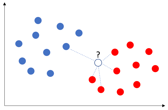
Figure (B) shows data points with the blue class and the red class. If there is a new data point, what should be the class for the new data point? The algorithm calculates the distances of this data point to other data points. For the 5-nearest neighbors, it counts the number of the blue and the red classes. In the graph, there are 4 red class and 1 blue class. The algorithm uses the majority voting rule to determine the class. The new data point is assigned the red class.
The procedure can be enumerated as below. In addition to Step 1 to 3 above, the supervised learning KNN does Step 4 and 5:
- Step 4: Among these K neighbors, count the number of the classes.
- Step 5: Assign the new data point to the majority class.
(C) How Is the Anomaly Score Defined?
Since an outlier is a point that is distant from neighboring points, the outlier score is defined as the distance to its kth nearest neighbor. Each point will have an outlier score. Our job is to find those points with high outlier scores.
The KNN method in PyOD uses one of the three types of distance measures as the outlier score: largest (default), mean, and median. The “largest” uses the largest of the distance to k neighbors as the outlier score. The “mean” and “median” use the average and median respectively as the outlier score.
(D) Modeling Procedure
I apply the following modeling procedure for the model development, assessment, and interpretation of the results.
- Model development
- Threshold determination
- Descriptive statistics of the normal and abnormal groups
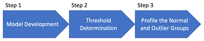
Step 1 will build the model and produce outlier scores. In Step 2, we will choose a threshold to separate the abnormal observations with high outlier scores from normal observations. If any prior knowledge suggests the percentage of anomalies should be no more than 1%, you can choose a threshold that results in approximately 1% of anomalies.
In Step 3, we will profile the two groups using the descriptive statistics (such as the means and standard deviations) by group. The descriptive statistic table is important to communicate the soundness of the model. If it is expected that the mean of a feature in the abnormal group is higher than that of the normal group and the result is counter-intuitive, you shall investigate, modify, or drop the feature. You shall reiterate Step 1 to 3 until the descriptive statistics of all features are consistent with expectations.
(D.1) Step 1: Build your Model
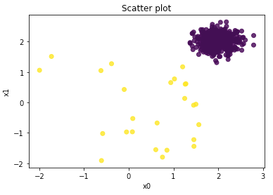
Let’s generate some data with outliers. I use the utility function generate_data() of PyOD and generate ten percent outliers. Notice that although this mock dataset has the target variable Y, the unsupervised KNN models only use the X variables. The Y variable is simply for validation.
The yellow points in the scatterplot are the ten percent outliers. The “normal” observations are the purple points.
The following code performs the computation for the k-NN model and stores it as knn. Notice that there is no y in the function .fit(). This is because y is ignored in the unsupervised methods. def fit(self, X, y=None). If y is specified, it becomes a supervised method.
The following code builds the model and scores the training and test data. Let’s review each line:
label_: This is the label vector for the training data. It is the same if you use.predict()on the training data.decision_scores_: This is the score vector for the training data. It is the same if you use.decision_functions()on the training data.decisoin_score(): This scoring function assigns the outlier score to each observation.predict(): This is the prediction function that assigns 1 or 0 based on the assigned threshold.contamination: This is the percentage of outliers. In most cases, we do not know the percentage of outliers so we can assign a value based on any prior knowledge. PyOD defaults the contamination rate to 10%. This parameter does not affect the calculation of the outlier scores.
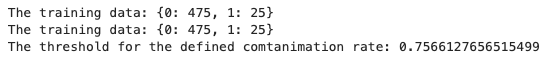
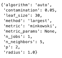
Let’s see the default parameters of KNN using .get_params(). The number of neighbors is 5.0. The contamination rate is set at 5%.
(D.2) Step 2: Determine a Reasonable Threshold
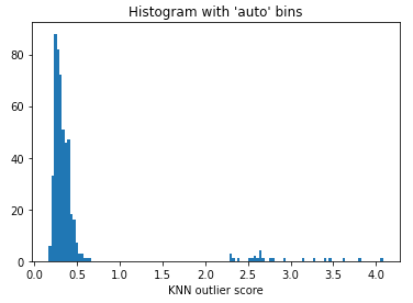
In most cases, we do not know the percentage of outliers. We can use the histogram of the outlier score to select a reasonable threshold. If there is any prior knowledge suggesting the anomalies to be 1%, you should choose a threshold that results in approximately 1% of anomalies. The histogram of the outlier score in Figure (D.2) suggests a threshold at 200.0 because there is a natural cut in the histogram. Most of the data points have low anomaly scores. If we choose 1.0 to be the cut point, we can suggest those >=1.0 are outliers.
(D.3) Step 3: Profile the Normal and Abnormal Groups
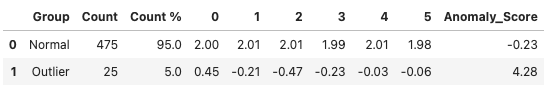
Profiling the normal and outlier groups is a critical step to demonstrate the soundness of a model. The feature statistics of the normal and the abnormal groups should be consistent with any domain knowledge. If the mean of a feature in the abnormal group should be high but the result is the opposite, you are advised to examine, modify, or discard the feature. You shall iterate the modeling process until all features are consistent with the prior knowledge. On the other hand, you are also advised to verify the prior knowledge if the data provide new insights.
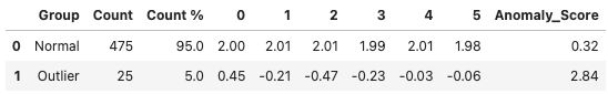
The above table presents the characteristics of the normal and abnormal groups. It shows the count and count percentage of the normal and outlier groups. You are reminded to label the features with their feature names for an effective presentation. The table tells us several important results:
- The size of the outlier group: Once a threshold is determined, the size is determined. If the threshold is derived from Figure (D.2) and there is no prior knowledge, the size statistic becomes a good reference to start with.
- The feature statistics in each group: All the means must be consistent with the domain knowledge. In our case, the means in the outlier group are smaller than those of the normal group.
- The average anomaly score: The average score of the outlier group should be higher than that of the normal group. You do not need to interpret too much on the scores.
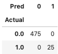
Because we have the ground truth in our data generation, we can produce a confusion matrix to understand the model performance. The model delivers a decent job and identifies all 25 outliers.
(E) Achieve Model Stability by Aggregating Multiple Models
KNNs can be sensitive to the choice of k. To produce a model with a stable outcome, the best practice is to build multiple KNN models and then aggregate the scores. This approach will reduce the chance of overfitting and increase prediction accuracy.
The PyOD module offers four methods to aggregate the outcome. You only need to use one method to produce your aggregate outcome.
- Average
- Maximum of Maximum (MOM)
- Average of Maximum (AOM)
- Maximum of Average (MOA)
I’ll create 20 KNN models for a range of k neighbors from 10 to 200.
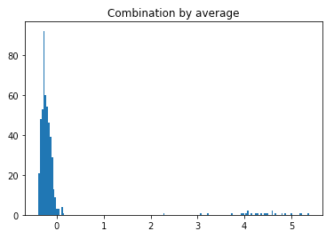
Figure (E) shows most of the data are below 0.0. There are a few outliers about 1.0. It probably makes sense to set the threshold at 1.0 or even 2.0. With that, we can profile the normal and outlier groups. The descriptive statistics are shown in Table (E). It identifies 25 data points to be the outliers. And the feature means of the outlier group are all smaller than those of the normal group. This is consistent to the results in Table (D.3).
(F) Summary
- The unsupervised k-NN method computes the Euclidean distance of observation to other observations. The unsupervised KNN does not have any parameters to tune to make the performance better. It simply computes the distances between neighbors.
- The outlier score of KNN is defined as the distance to its kth nearest neighbor.
(F) Python Notebook: Click here for the notebook.
Appendix: What Are the “Distances” in kNN and k-Means?
kNN finds the distance to the nearest neighbors, and k-Means find the distance to the centroid of a cluster.
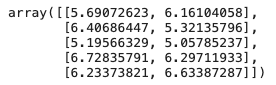
The Scikit-learn library includes the supervised kNN (See 1.6.1 Unsupervised Nearest Neighbors) and the K-means algorithm. I am going to use only the top five data points from our data to show you the differences.
(F.1) k-NN:
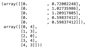
The unsupervised k-NN computes the distance of a point to its nearest data point. For example, the nearest point of point ‘0’ (notice Numpy labels the five points as [0,1,2,3,4]) is point 4, and the distance is 0.72002248.
(F.2) k-means:
When you specify there will be N clusters. The k-Means method starts with N randomly chosen seeds. It computes the distance of each data point to those N seeds. Then k-means assigns each data point to the nearest seed to form a cluster. This will group the data points into N clusters. Then k-means updates each seed location with the centroid of the cluster, thus the seed is the centroid of the cluster. This process will be iterated until the values of the centroids stabilized.
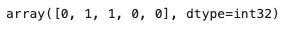
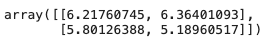
The above output shows the clusters of the five points. And the output below shows the locations of the centroids in the two clusters.
For easy navigation to chapters, I list the chapters at the end.
- Chapter 1 — Introduction
- Chapter 2 — Histogram-Based Outlier Score (HBOS)
- Chapter 3 — Empirical Cumulative Outlier Detection (ECOD)
- Chapter 4 — Isolation Forest (IForest)
- Chapter 5 — Principal Component Analysis (PCA)
- Chapter 6 — One-Class Support Vector Machine (OCSVM)
- Chapter 7 — Gaussian Mixed Models (GMM)
- Chapter 8 — K-nearest Neighbors (KNN)
- Chapter 9 — Local Outlier Factor (LOF)
- Chapter 10 — Clustering-Based Local Outlier Factor (CBLOF)
- Chapter 11 — Extreme Boosting-Based Outlier Detection (XGBOD)
- Chapter 12 — Autoencoders
- Chapter 13 — Under-sampling for Extremely Imbalanced Data
- Chapter 14 — Over-sampling for Extremely Imbalanced Data
Readers are recommended to purchase books by Chris Kuo:

- The explainable AI: https://a.co/d/cNL8Hu4
- Transfer learning for image classification: https://a.co/d/hLdCkMH
- Modern time series anomaly detection: https://a.co/d/ieIbAxM
- Handbook of Anomaly Detection: https://a.co/d/5sKS8bI


