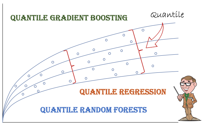
A Tutorial on Quantile Regression, Quantile Random Forests, and Quantile GBM

Have you been asked to provide prediction intervals beside the mean predictions? Prediction intervals have many use cases because they provide the range of the predicted values to give better guidance. In financial risk management, the prediction intervals for the high range can help risk managers to mitigate risks. In science, a predicted life of a battery between 100 to 110 hours can inform users when to take action. Please comment on which of the following is more applicable.

• The expected average financial loss is $40M, or
• We have 95% confidence that the financial loss will be between $10M and $70M, with an average of around $40M. Further, we have 68% confidence that the financial loss will be between $30M and $50M.

The second one, right? The first one is the prediction of an Ordinary Least Square (OLS) and the second one is a Quantile Regression (OR). For this reason, QR has received increasing attention and applied to many areas such as investment, finance, economics, medicine, and engineering.

An OLS only predicts the conditional mean Y = E[Y|X]+e. If OLS models the conditional means, why don’t we model the conditional median or any other percentiles (the term quantile in QR is the same as a percentile)? It is interesting to know that QR was invented about the same time as the ordinary least square (OLS) but becomes popular due to today’s good computational power.

What are the advantages of QR?

QR is attractive for the following reasons:

• First, QR models the entire conditional distribution of the target variable, while OLS only delivers the mean estimates.
• Second, QR does not assume the target distribution, so is more robust to misspecification of the error distribution.
• Third, QR is not sensitive to outliers. OLS estimates the conditional mean so is sensitive to outliers.
• Fourth, QR is invariant to monotonic transformations, such as log(·), so the quantiles of h(y), a monotone transform of y, are h(Qq(y)), and the inverse transformation may be used to translate the results back to y.

Most machine learning (ML) techniques such as Random Forest or Gradient Boosting only provide the mean prediction. Won’t it be great if these ML techniques can deliver quantile measures? In this post I will walk you through step-by-step Quantile Regression, then Quantile Gradient Boosting, and Quantile Random Forests. I also have made the entire notebook available on GitHub. If you need good computational power, you can consider using Google Colab to run the code. See “Start Using Google Colab Free GPU”.

Dataman has published a wide range of data science articles from feature engineering to model adoption and SHAP values, from deep learning to NLP, and from econometrics to industry use cases. You are recommended to bookmark “Dataman Learning Paths — Build Your Skills, Drive Your Career”. It may be CPU- and time-consuming to run Quantile Random Forests

(A) When Should You Use QR?

When you are interested in the prediction intervals, or the distribution of the target variable is heteroscedastic, you are recommended to use QR. This is because QR does not make assumptions about the distribution of the target variable.

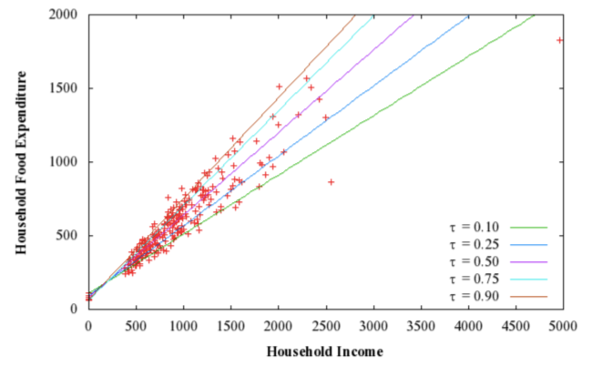
Figure (A) shows an example from Koenker R (2005) Quantile Regression Econometric Society Monographs, Cambridge University that household food expenditure varies even more widely for high-income households. An OLS gives the prediction for the mean, but it is often needed to estimate the range of the variance.

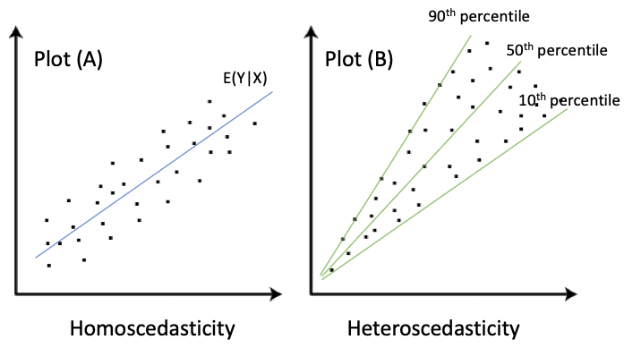
Let me use two plots to explain. Plot (A) below shows the case that the variance of Y stays the same, and in Plot (B), the variance of Y increases as X increases. In Econometrics, Plot (A) is called homoskedasticity, in which the variance of the residual term remains constant. Plot (B) is called heteroscedasticity, in which the variance varies widely. Most real-world data would look like Plot (B) rather than Plot (A). OLS regression assumes homoskedasticity. Thus QR becomes more appealing when heteroscedasticity exists.

Prediction Interval Is Different from Confidence Interval

Before I introduce QR, I like to clarify that the prediction Interval is different from the confidence interval, and the prediction interval is wider than the confidence interval. A confidence interval tells you the range of a coefficient, such as 𝜷±1.96 S.E.(𝜷) in a regression. Prediction intervals tell you the interval where a future value will fall.

(B) Let’s Use A Data Example

I will use the Boston house price dataset. This dataset contains information collected by the U.S Census Service concerning housing in the area of Boston, Massachusetts. It has been used extensively throughout the literature to benchmark algorithms. It has 506 rows and 14 columns. This popular dataset has many sources and is even included in the scikit-learn datasets for practice purposes. Although this post claims some issues with the data, I found those issues are unrelated to this post.

The goal is to predict the median house value (MEDV) with the following variables.

• MEDV: (Target) median value of owner-occupied homes in \$1000s.
• CRIM: per capita crime rate by town.
• ZN: proportion of residential land zoned for lots over 25,000 sq. ft.
• INDUS: proportion of non-retail business acres per town.
• CHAS: Charles River dummy variable (= 1 if tract bounds river).
• NOX: nitrogen oxides concentration (parts per 10 million).
• RM: average number of rooms per dwelling.
• AGE: proportion of owner-occupied units built before 1940.
• DIS: weighted mean of distances to five Boston employment centers.
• RAD: index of accessibility to radial highways.
• TAX: full-value property-tax rate per \$10,000.
• PTRATIO: pupil-teacher ratio by town.
• BLACK: 1000(Bk — 0.63)² where Bk is the proportion of blacks by town.
• LSTAT: lower status of the population (percent).

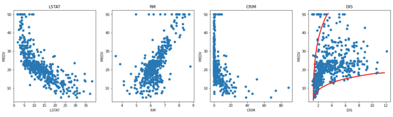
The plots below show the relationships between MEDV and a few variables. Some plots already exhibit heteroscedasticity.

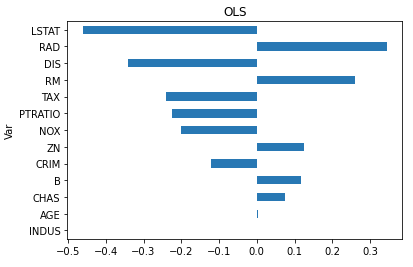
(C) Let’s Start with OLS

People often state loosely that “an OLS models the mean”. It should be stated formally as the conditional mean. The conditional mean of Y given X=x is defined as E[Y|X=x]. The following code fits an OLS model. It results an R-squared of 0.73. I plot the variables in descending order: “LSTAT” has the strongest influence on the mean of Y, followed by “RAD”, “DIS” and so on.

(D) Quantile Regression

The above OLS provides only a partial view of the relationships between X and Y. We might be interested in describing the relationship at various points in the conditional distribution of y. I am interested in the 1%-, 5%-, 50%- (median), 95%-, and 99%-percentile of the target variable (imagine five lines in Plot (B)). Because I list five percentiles, there will be five Quantile Regressions. Since there are five different models, the variable coefficients shall vary. It will be fascinating to see how the variables vary from quantile to quantile.

I make the function Qreg to perform modeling, and compute the coefficients with lower and upper bounds. I store the coefficients of the five models in Qreg_coefs. The R-squared value of the 50%-percentile is 0.75.

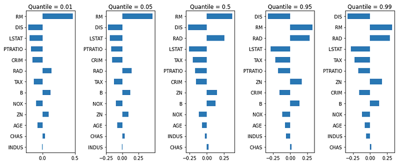
The coefficients of the five quantile regression models are plotted in bar charts. The coefficients are ranked in descending order by their absolute size.

The most fascinating result is the variable ranking in the five quantile regression models can vary. The 50%-percentile model (in the middle) tells us “RM”, “DIS” and “RAD” are the most influential variables. However, the 1%-percentile model has “LSTAT” in the 3rd place, and the 99%-percentile model has “DIS” in the 1st place.

(E) How Does Quantile Regression Work?

QR uses Least-Absolute-Deviation (LAD) to obtain the estimators. To explain how it works, we will start with OLS, then Median regression, and extend to Quantile Regression. We know a linear model Y = X 𝛃 + e minimizes the sum of squared errors to obtain the best estimator:

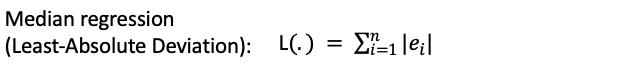
A Median Regression minimizes the Absolute Deviation to obtain the estimator. It is called the Least Absolute Deviation. If X is symmetric, the mean and median will be approximately the same and the estimator will be the same as that of the OLS.

The idea of the least-absolute-deviation (LAD) regression is just as straightforward as that of an OLS. However, LAD regression does not have an analytical solving method like that of an OLS. Linear programming or the simplex method is required. It searches for the estimator that satisfies the following requirement:

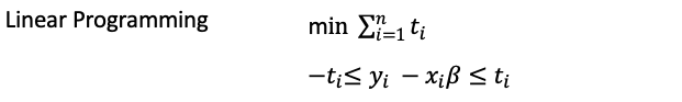
Today’s computational power has made linear programming very easy. This EXCEL-based approach demonstrates how to perform LAD. Further, this LAD can be extended to the following quantile regression estimator.

Quantile regression minimizes a sum that gives asymmetric penalties (1 − q)|ei | for over-prediction and q|ei | for under-prediction. When q=0.50, the quantile regression collapses to the above equation.

(F) Quantile GBM

Modern machine learning algorithms have incorporated the quantile concept. The scikit-learn function GradientBoostingRegressor can do quantile modeling by loss='quantile' and lets you assign the quantile in the parameter alpha.

alpha = 0.95

clf = GradientBoostingRegressor(loss='quantile', alpha=alpha)

I make the function GBM() below to perform both the modeling and prediction. I store the five models in GBM_models and the predictions in GBM_actual_pred. (The same structure will be repeated in the Quantile Random Forests. I purposely made this similarity so it is easy for readers to follow.)

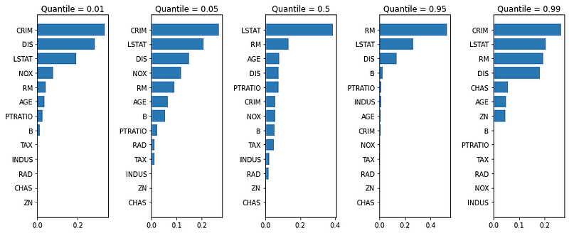
Five GBM models were built: the 1%-, 5%-, 50%-, 95%-, and 99%-percentile. Again, we see the variables rank differently in the five models. The 50%-percentile GBM model (in the middle) tells us “LSTAT”, “RM” and “AGE” are the most influential variables. The 1%-percentile (99%-percentile) model shows “CRIM”, “DIS”, and “LSTAT” (“CRIM”, “LSTAT” and “RM”) are the top three variables. You can inspect all other models.

The following code also shows the R-squared is .89, compared with 0.73 in OLS, and 0.75 in Quantile Regression.

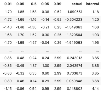
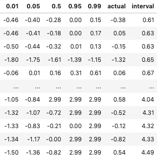
The table below are some examples inGBM_actual_pred. It is expected that most actual values shall fall inside the 1% and 99% intervals. Can we verify that?

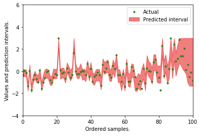
Do most of the actual values fall inside the 1% and 99% intervals? The plot shows the prediction intervals and the actual values.

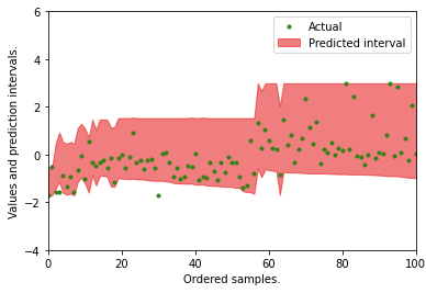
Another way to measure the prediction outcome is to count how many observations fall within the intervals. The following function does that and gets 96.07%.

(G) Quantile Random Forests

The standard random forests give an accurate approximation of the conditional mean of a response variable. Nicolai Meinshausen (2006) generalizes the standard random forests to provide information for the full conditional distribution of the response variable, not only about the conditional mean. Therefore quantile regression forests give a non-parametric and accurate way of estimating conditional quantiles for high-dimensional predictor variables.

How does it work? The standard random forest model calculates the mean value of the target variable in each tree leaf. If we record all observed responses in the leaf, we will be able to calculate the percentiles. Assume in a random forest model there are 100 trees, which produce 100 predicted values for an input observation. The standard random forests get the conditional mean by taking the mean of the 100 predicted values. We can extend this to get the entire distribution thus the confidence intervals.

I want to emphasize here that this approach does not build five quantile random forest models, as the Quantile GBM did. The solution here just builds one random forest model to compute the confidence intervals for the predictions. We will not see the varying variable ranking in each quantile as we see in the above Quantile GBM, we still can deliver the prediction intervals.

The code below builds 200 trees. It “unpacked” the random forest model to record the predictions of each tree. The predictions of the 200 trees for an input observation are stored in the 200 columns. I have made it efficient that the predictions of a tree are for all observations in a list. The time-consuming part is the number of trees. You are advised to find the minimum number of trees first.

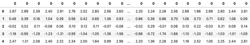
How to get the prediction intervals for each observation (row)? What we need to do is to compute the percentile statistics by column. This can be done fairly efficiently in pandas.

In addition, we have two numbers to measure the outcome. The first one is R-squared. We got R-squared = 0.81. This is in line with GBM’s .89, OLS’s 0.73, and QR’s 0.75. The second one is the percentage of the actuals falling inside the 1% and 99%. We got 95.9%, close to GBM’s 96.07%.

Although scikit-learn has the class skgarden to import RandomForestQuantileRegressor, it suffers glitches at the time I am writing this post. So I do not use skgarden in this article.

You are encouraged to download the notebook from this Github.

(H) H2O Quantile GBM & Quantile Deep Learning

H2O also offers the algorithms for the quantile GBM and the quantile Deep Learning. Click this H2O page to test it out.

H2O has proven to be one of the favorite tools of many data scientists. It streamlines modeling development and production and can produce models that can be run in other languages such as Java. If you are new to H2O, you will get a great start by reading “My Lecture Notes on Random Forest, Gradient Boosting, Regularization, and H2O.ai”.