Algorithmic Trading with Technical Indicators in R

Feature engineering is one of the fun, creative, and essential steps in machine learning. It transforms raw data into a form of very meaningful information for a model to forecast the future. The predictability of a model relies on good features, which in turn relies on your domain knowledge.

Many experienced stock market traders who evaluate trading rules or charts have already engaged in some form of feature engineering — whether they realized it or not. For example, a moving average is a feature that characterizes the movement of a stock price. All the technical indicators (RSI, MACD, stochastic oscillators, Bollinger Bands, etc.) are some forms of features too. These features can be fed into a machine learning model, or used as trading signals. There can be hundreds, if not thousands, of trading strategies to capture market anomalies or predict future trends.

In this post I will walk you gently to build your algorithmic trading code in R. R has several powerful quantitative finance libraries because of its long development history including quantmod, TTR, and PerformanceAnalytics. If you are new to algorithmic trading, you will be ready to start your algorithmic trading. You can download the code from this GitHub.

Time Series Articles

If you are interested in a comprehensive survey on time series forecasting and anomaly detection, below is a list that you may find helpful:

• Part 1: “Anomaly Detection for Time Series“
• Part 2: “Detecting the Change Points in a Time Series”
• Part 3: “Algorithmic Trading with Technical Indicators in R”
• Part 4: “Kalman Filter Explained!”
• Part 5: “Business Forecasting with Facebook’s “Prophet”
• Part 6: “Time Series with Zillow’s Luminaire — Part I Data Exploration”
• Part 7: “Time Series with Zillow’s Luminaire — Part II Optimal Specifications”
• Part 8: “Time Series with Zillow’s Luminaire — Part III Modeling”
• Part 9: “A Technical Guide on RNN/LSTM/GRU for Stock Price Prediction”

Part 9 applies a Recursive Neural Network (RNN), Long Short-Term Model (LSTM), and Gated recurrent unit (GRU) in stock price prediction with decent performance. You are advised to read that article if you are looking for a thorough technical guide. Also, you may want to develop a web service for your stock price prediction service. If you are a Python user, you may be thinking of Flask or Django as your web-service frameworks. I highly recommend Streamlit in Python, as I explain in “Building a Stock Market App with Python Streamlit in 20 Minutes”.

(0) The Four-Decade Debates on Market Efficiency

As we discuss the efficacy of algorithmic trading or technical rules, the iconic debates on the “efficiency market hypothesis” (EMH) always come to our minds. Although this article does not plan to address the debate, it is worthwhile to mention it here. It is believed that prices should already fully reflect all available information. There is no way to “beat the market” to obtain abnormal returns. According to EMH, prices already reflect at least all past publicly available information — so-called the weak form; or prices change instantly to reflect all publicly available information — so-called the semi-strong form; or prices have also reflected any hidden insider information — so-called the strong form. Eugene Fama, the 2013 Nobel Prize winner, believes anomalies are consistent with rational pricing.

Do all traders subscribe to the EMH? Not really. Many traders believe there exist opportunities that prices are mis-priced and they can obtain abnormal returns. An “anomaly” is a situation that a price does not fully reflect all the public information, thus providing a trading opportunity. Although “beating the market” is something many novice or experienced traders try to do, few succeed. Robert Shiller –also a 2013 Nobel Prize winner — believes that markets are irrational and subject to behavioral biases in investors’ expectations. If that is the case, investment performance can be improved by advanced predictive models that are always in place or yet to come. Readers who are interested in the philosophical debates and empirical verifications, please see my post “Stock Market Anomalies” and “Stock Market Anomaly Detection” Are Two Different Things.

Okay. Now is the time to enjoy coding for algorithmic trading.

(A) R’s Power Tools for Finance:

The “quantmod”, “TTR” and “PerformanceAnalytics” libraries are the three most used R libraries for quantitative finance, while more libraries are being developed. These libraries let you focus on testing various trading strategies. Use getSymbols() to download the historical data of a symbol. Also, getSymbols uses the symbol name as the dataset name.

(B) Stock Data Transformation

(B.1) Returns between Open, High, Low, and Close

These handy functions make your calculation easy. OpCl computes the return from Open to Close; Opop, from Open to Open; HiCl, from High to Close, etc. I print out the results so you can see how they work.

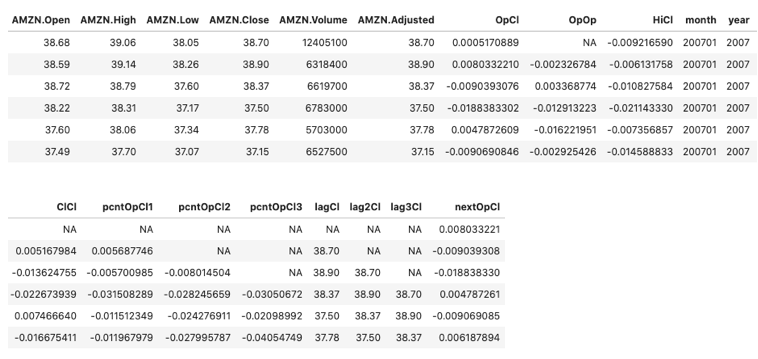
Let me explain the above columns:

• OpCl: is quantmod’s function to calculate the percentage change from the open price to the close price of the same day.
• OpOp: is quantmod’s function to calculate the percentage change for the open prices between two days.
• HiCl: it calculates the percentage change from the high price to the close price of the same day.
• ClCl: it calculates the percentage change for the close prices between two days.
• pcntOpCl1: I use the R function Delt() to calculate the percentage change between the open price of Day x and the close price of Day x+1 (the next day).
• pcntOpCl2: this calculates the percentage change between the open price of Day x and the close price of Day x+2 (two days later).
• pcntOpCl3: this calculates the percentage change between the open price of Day x and the close price of Day x+3 (three days later).

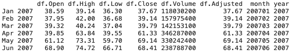
(B.2) To Weekly or Monthly

Often you need to reduce the daily stock records to weekly or monthly stock records. The irregularities in a calendar, such as holidays, leap year, or months of the year, will drive your programming crazy. The handy R functions like to.monthly or to.weekly will save much of your time.

(B.3) Daily, Weekly, and Monthly Returns

Likewise, these R functions can calculate the stock returns easily.

(C) Understand the Basic Characteristics of Stock Returns

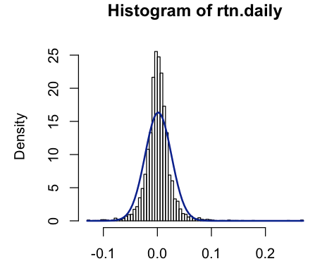
It is well-known that the distributions of daily and monthly stock returns are fat-tailed relative to the normal distribution. The shape of their return distribution is more peaked than a symmetric, bell-shaped, standard normal distribution. It means extreme events (a large price move) are more likely to happen than a standard normal curve.

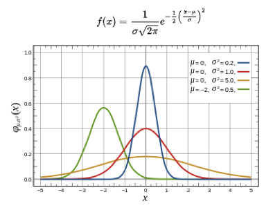
Kurtosis (from Greek: κυρτός, kyrtos or kurtos, meaning “curved, arching”) measures whether a distribution is heavy-tailed or light-tailed relative to the standard normal distribution. A heavy-tailed distribution looks like the blue curve in Figure C — it is tall in the center and stretched very far in the two ends (thus heavy-tailed). Higher kurtosis corresponds to the greater extremity of deviations (or outliers). Note that while it is convenient to remember high kurtosis corresponding to a tall curve, it is technically incorrect to say kurtosis measures the “peakedness” of a curve. Below I plot the distribution of stock returns to a standard normal distribution.

• A standard normal distribution has 0 means, 1 standard deviation, and 0 excess kurtosis
• The distribution of typical stock returns has a small standard deviation and positive excess kurtosis.

(D) Frequently-Used Technical Analysis (TA) Indicators

(D.1) MACD — Moving Average Convergence Divergence

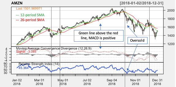
The MACD was developed by Gerald Appel and is probably the most popular price oscillator. It can be used as a generic oscillator for any univariate series, not only price. Typically MACD is set as the difference between the 12-period simple moving average (SMA) and 26-period simple moving average (MACD = 12-period SMA − 26-period SMA), or “fast SMA — slow SMA”.

• The MACD has a positive value whenever the 12-period SMA is above the 26-period SMA and a negative value when the 12-period SMA is below the 26-period SMA. The more distant the MACD is above or below its baseline indicates that the distance between the two SMAs is growing.
• The MACD function in R also computes the moving average of the MACD, called the signal. The default number of periods to compute the signal is nine periods.

Why are the 12-period SMA called the “fast SMA” and the 26-period SMA the “slow SMA”? This is because the 12-period SMA reacts faster to the more recent price changes, than the 26-period SMA.

(D.2) What does the MACD look like?

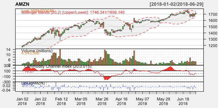
The MACD line oscillates around 0. When the fast SMA is above the slow SMA, the MACD is above 0, and vice versa. As shown in Figure (I), the green line is the fast SMA and the red line is the slow SMA. The four vertical lines are where the fast SMA crosses the slow SMA, or in other words, where the MACD crosses 0. The dashed line around the MACD is the signal line, which is the 9-period simple moving average of MACD.

(D.3) RSI — Relative Strength Index

Introduced by Welles Wilder Jr. in his seminal 1978 book “New Concepts in Technical Trading Systems”, the relative strength index (RSI) becomes a popular momentum indicator. It measures the magnitude of recent price changes to evaluate overbought or oversold conditions. It is displayed as an oscillator and can have a reading from 0 to 100. The general rules are:

• RSI >= 70: security is overbought or overvalued and may be primed for a trend reversal or corrective pullback in price.
• RSI <= 30: an oversold or undervalued condition.

The formula of RSI is a little bit complex. See here for the definition.

(D.4) What does the RSI look like?

The bottom section in Figure (I) is the RSI line, which is shown in blue. Notice there are some incidences where the price drops dramatically so the RSI is below 30, pointed out as “oversold” in Figure (I).

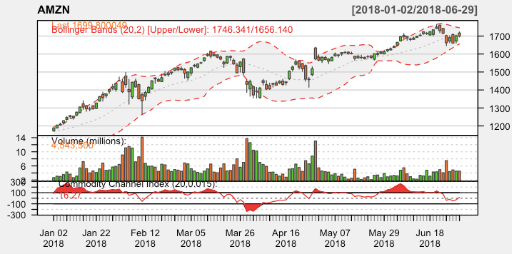
(D.5) Bollinger Bands

The Bollinger Bands are a type of price envelope developed by John Bollinger. They are envelopes plotted at a standard deviation level above and below a simple moving average of the price. Because the distance of the bands is based on standard deviation, they adjust to volatility swings in the underlying price. Bollinger bands help determine whether prices are high or low on a relative basis. They are used in pairs, both upper and lower bands, and in conjunction with a moving average. Further, the pair of bands is not intended to be used on its own. Use the pair to confirm signals given with other indicators. Bollinger Bands use 2 parameters, Period and Standard Deviations, StdDev. The default values are 20 for the period, and 2 for standard deviations, although you may customize the combinations. “Distance from a moving average” or “standard deviation” apply the same concept. Click here for more detail.

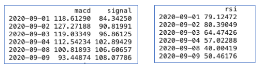
Below I use the MACD and RSI functions in “TTR” to generate the technical indicators. You are encouraged to experiment with all other technical indicator functions. The dataset “macd” has two columns: macd and its 9-period moving average called ‘signal’.

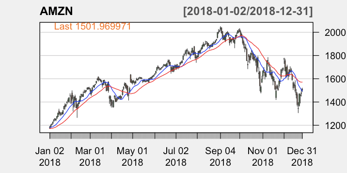
(E) How to Plot Technical Charts

The following few lines let you generate professional stock charts and add many technical indicators to the charts. The “quantmod” library includes more than 30 technical indicators.

(F) Develop Your Trading Strategies and Signals

The general idea of algorithmic trading is to enter and stay in the market when it is a bullish market and exit when it is a bearish market. The bullish market is typically when the 12-period SMA crosses the 26-period from below. This is the same as the MACD line crosses zero, and MACD is higher than the signal line. The bearish market is when the 12-period SMA dives below the 26-period SMA.

You can form many trading strategies with various combinations of technical indicators. Below I demonstrate three strategies and the Buy-and-hold strategy.

(F.1) Strategy 1:

• Enter and stay in the market when MACD>Signal, and
• Otherwise

(F.2) Strategy 2: overbought trend

We can add RSI to our strategy. An overbought stock (RSI > 70) may indicate rising price opportunities. So our strategy becomes:

• Enter and stay in the market when MACD>Signal and RSI>70,
• otherwise

(F.3) Strategy 3: oversold for rebound opportunity

An oversold stock (RSI < 30) may indicate a price rebound opportunity. So our strategy becomes:

• Enter and stay in the market when MACD
• otherwise

(F.4) The Buy-and-hold strategy

Let’s code these strategies:

(G) Backtesting

Backtesting is a critical step before implementing a strategy. Without this, a trader wouldn’t even consider entering the markets. Backtesting applies a trading strategy or analytical method to historical data to see how accurately the strategy or method would have been predicted. The need to backtest is intuitive. Before you buy a Laptop or a book, don’t you want to check its brand, its functionalities, or other users’ comments? The same idea applies to stock market trading. Although there are many exceptions that backtesting is not always true, it is still the biggest advantage of Algorithmic Trading.

(G.1) What to track in backtesting:

The essential metrics in backtesting include the cumulative returns, the annualized returns, the Sharpe ratio, and the annualized Sharpe ratio. The Sharpe ratio was developed by Nobel Laureate William Sharpe. It measures the performance of an investment compared to a risk-free asset, i.e., after adjusting for its risk. It is defined as the difference between the returns of the investment and the risk-free return, divided by the standard deviation of the investment (i.e., its volatility):

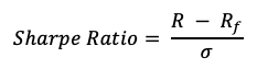
The R library “PerformanceAnalytics” defaults the risk-free return to zero if the risk-free rate is not specified.

(G.2) How to Use the Sharpe Ratio?

The higher a fund’s Sharpe ratio, the better a fund’s returns have been relative to the risk it has taken on. Because it uses standard deviation, the Sharpe ratio can be used to compare risk-adjusted returns across all fund categories.

The higher a fund’s standard deviation, the higher the fund’s returns need to be to earn a high Sharpe ratio. Keep in mind that even though a higher Sharpe ratio indicates a better historical risk-adjusted performance, this doesn’t necessarily translate to a lower-volatility fund.

(G.3) Backtesting Code

I write the following function to perform backtesting, which returns the four elements. Notice the input “strategy” is lagged by one period. Why do I do that? It is because when you see the daily returns, the market is already closed. Your trading has to take place on the next day.

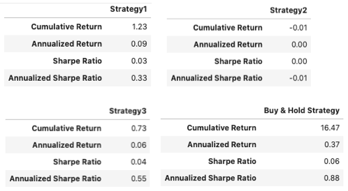
The above results show the Buy-and-Hold strategy is far better than my trading strategy for Amazon stock. Interesting isn’t it? The buy-and-hold strategy has been criticized for years, yet its performance still is proven for some selected stocks.

To save time, you can download the code from this GitHub.

Readers are recommended to purchase books by Chris Kuo:

• The explainable AI: https://a.co/d/cNL8Hu4
• Transfer learning for image classification: https://a.co/d/hLdCkMH
• Modern time series anomaly detection: https://a.co/d/ieIbAxM
• Handbook of Anomaly Detection: https://a.co/d/5sKS8bI