
Anomaly Detection for Time Series

The local beach is not far from where I live, so sometimes I go there to enjoy my solitude. I watch the ocean waves come and go, leaving a belt of wet sand. I watch my footprints along the wet sand appear and disappear. One day I had an aha moment. These footprints are like the data points in a time series, and the belt of the wet sand is the acceptable range by a time series model. There are a few footprints outside the belt called anomalies or outliers. When the belt covers the normal footprints, none of them is anomalous. But when the belt moves, some footprints are exposed outside the belt and become anomalies.
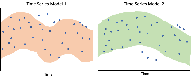
This ocean stroll reminds me of the challenge of building a time series model to identify anomalies accurately. The challenges are: (i) considering anomalies as normal footprints, and (ii) considering normal footprints as anomalies. Figure (I) shows one model may consider data as anomalous but another model may not. How do we tackle these challenges? I know the following two steps are essential: (1) understanding the data patterns and source of noises, and then (2) choosing suitable techniques.
Data patterns are patterns that have happened in the past and are likely to repeat in the future. How do you find them? Data patterns can be captured by feature engineering. Many time series such as electricity consumption data and telemetry data follow fixed periodical patterns. You can create features such as the hour of the day and the day of the week to capture fixed periodical patterns. Is this the first time that you've heard the term telemetry? Telemetry data is the automated collection of data through devices such as home security devices, medical devices, or agricultural surveillance aircraft. Anomaly detection for telemetry data becomes increasingly important as our lives are surrounded by telemetry data.
Other complex time series like stock price time series or macroeconomic time series may not follow a fixed periodical pattern. For example, in “Algorithmic Trading with Technical Indicators in R” or “Practical algorithmic trading — (1) Why algo trading and technical indicators?”, I show all the technical indicators (RSI, MACD, stochastic oscillators, Bollinger Bands, etc.) are some forms of features that can capture data patterns.
In this post, I will walk you through the popular techniques for time series anomaly detection from simple to complex. I will start with the concept of a tolerance band, then cover the moving average techniques, and then seasonal-trend decomposition for the fixed patterns. The notebook of this post is available through this link. Once you complete the current article, you are advised to read through the following sequence. You will gain strong time series knowledge in this series.
- Part 1: “Anomaly Detection for Time Series“
- Part 2: “Detecting the Change Points in a Time Series”
- Part 3: “Algorithmic Trading with Technical Indicators in R”
- Part 4: “Kalman Filter Explained!”
- Part 5: “Business Forecasting with Facebook’s “Prophet”
- Part 6: “Time Series with Zillow’s Luminaire — Part I Data Exploration”
- Part 7: “Time Series with Zillow’s Luminaire — Part II Optimal Specifications”
- Part 8: “Time Series with Zillow’s Luminaire — Part III Modeling”
- Part 9: “A Technical Guide on RNN/LSTM/GRU for Stock Price Prediction”
(0) Determine the tolerance band
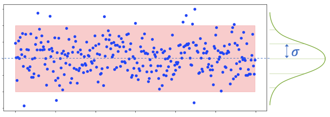
The width of the band matters: a narrow band may consider too many points as anomalous, and vice versa. How do we determine the width? Time series usually follow a normal distribution in which the center, or called the mean, has more data points. You can calculate the standard deviation of your predicted time series. In a normal distribution, approximately 68% (95%) of the data points fall inside one (two) standard deviations away from the mean. However, you are advised not to take the number of standard deviations as a hard rule. This is because the distribution of a time series may not closely follow a standard normal distribution, and your model is an approximation that may not capture the source of the patterns precisely. You still need to inspect the outliers with the users to determine an acceptable level of width.
In this post, I use the Bike Share Daily data from Kaggle which you can find from here. The bike-sharing daily count is highly correlated to weather conditions and seasonality (day of week and season).
(1) Simple Moving Average
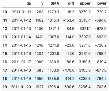
The simple moving average (SMA) is a quick way to capture the pattern in a time series. It is merely the mathematical average of the past N data points. It can be done with .rolling(window=N).mean() like below.
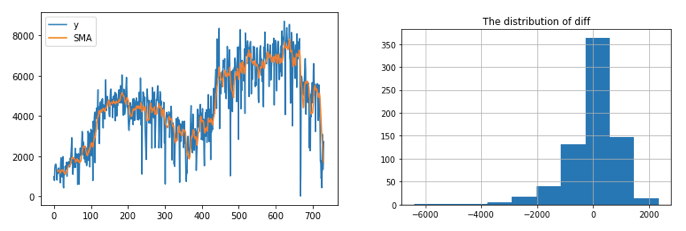
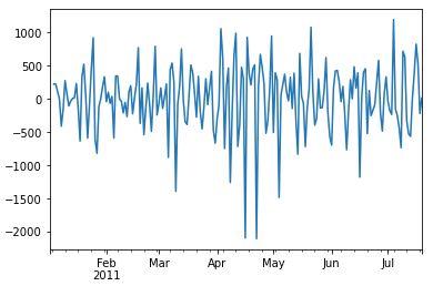
I calculate the differences between the actual and the simple moving average. The histogram shows the majority of the data are above or below the SMA by about 2,000.
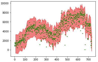
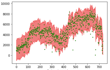
The code below plots the tolerance band and has revealed the outliers.
The SMA method smooths the rough edges in a time series to identify the pattern. It is the simple average of the data in the chosen time window. It does not put more weight on recent data and less weight on remote data. However, it may be more intuitive to do as we just argued. Let me introduce another smoothing method: exponential smoothing.
(2) Exponential Smoothing
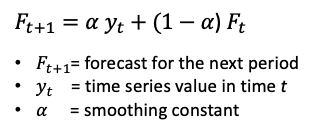
Exponential Smoothing is a very popular scheme to produce a smoothed Time Series. Recall in Single Moving Averages the past observations are weighted equally. But isn’t it more intuitive that recent data points should have a stronger influence on today’s data than ancient data? Exponential Smoothing is designed to address this problem. Exponential Smoothing assigns exponentially decreasing weights as the observation gets older. In other words, recent data are given relatively more weight in forecasting than older data.
In the case of moving averages, the weights assigned to the observations are the same and are equal to 1/N. In exponential smoothing, however, there are one or more smoothing parameters to be determined (or estimated) and these choices determine the weights assigned to the observations. The equation is:
Line 8: It generates a smoothed curve given the smoothing factor = 0.2 and does not try to optimize the factor value by setting optimized=False. This example demonstrates an example that optimizes the factor value by setting optimized=True.
Line 9: It generates forecasts for the next three periods. It gives a label for this time series that the factor value is 0.2.
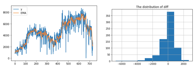
In our example, the predictions and the histogram of the EMA happen to be very similar to those of the SMA. I also use 2000 to get the tolerance band.
The above two methods are “quick” models that do not analyze and models the source of the patterns. As we inspect more carefully, we may realize that the events in the data are calendar-driven and can be modeled accordingly. So let’s re-consider a time series.
(3) Let’s Consider a Hypothetical Time Series
A univariate time series is a function of time. Other than time itself, we do not use other covariates to predict the movement of the time series. It could be the case that we may not have other covariates to forecast the target time series, or the time series itself just follows strongly calendar effects. By capturing the major calendar effects, we can forecast the cyclical movements. It is granted that there will be many factors resulting in the fluctuation of a time series. The modeling goal is not to identify a cyclical pattern as an unexpected noise, nor to identify noise as a fixed pattern.
Consider the hypothetical time series in Figure (D). It says the peaks and the valleys are the results of certain days in a week, months in a year, or holidays. If the time series exhibits a general uptrend, it may be due to the overall trend effect. None of these should be considered abnormal. If we can identify the major components of these factors, we shall be able to build an explicit univariate model to forecast the future. Any deviations to the forecasts can be considered anomalies.
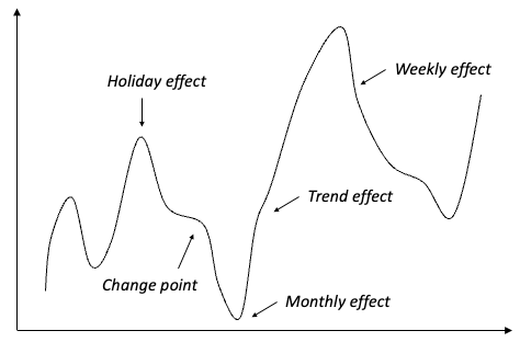
Notice that in Figure (3) there is an important effect “change point”. A change point is a past one-time known event and will not repeat in the future. The failure to identify those change points will incorrectly reproduce the one-time event in the future. Many time series models including Prophet in Part 5: “Business Forecasting with Facebook’s “Prophet” and Luminaire in Chapters 6–8 can detect past change points. For this reason, the topic “change point detection” is arranged before Chapter 5 to give us a thorough theoretical and practical understanding.
(3) Seasonal-Trend Decomposition (STD)
This technique gives you the ability to split your time series signal into three parts: seasonal, trend, and residual, and is suitable for many time series that possess calendar patterns. This model assumes the three components are simply additive, meaning you can simply add them up to get back to the original time series (seasonal + trend + residual = the time series). The algorithm automatically searches for the periodical patterns.
Let me print each of the three components.
It is intuitive to split a time series into the above three components, but the mathematical additive assumption may be too strong and too restrictive. How can we make an algorithm that applies the same idea, but relax the strict additive assumption a little bit? It is what I am going to introduce to you — the “prophet” module based on the general additive model assumption.
(4) The Prophet Module
The prophet module is open-sourced by Facebook.com and available in both R and Python. If a time series can be formulated by the time such as year, season, month, or week, the prophet module is a good choice. The model assumes a general additive model (GAM) that a time series can be specified with the following components:
y(t) = g(t) + s(t) + h(t) + ε(t)
- Trend: g(t),
- Seasonality: s(t) for weekly and yearly seasonality,
- Holiday Effects: h(t) for the effects of holidays that occur on potentially irregular schedules over one or more days,
and ε(t) is for any idiosyncratic changes which are not accommodated by the model. The predictor is t or time.
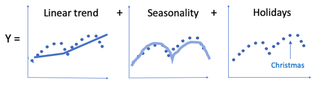
If the above functions g(t), s(t), and h(t) are linear, the model becomes a Seasonal-Trend Decomposition model. That’s why the GAM provides more flexibility than the STD model. It means the trend or seasonality pattern can contribute to the predicted values y(y) in any functional form such as piecewise linear or segmented function in the above “Linear trend” sub-graph.
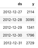
Do pip install prophet or pip install fbprophet. The prophet module requires two columns with the name “ds” and “y”. The bike ride time series is daily, so Line 13 specifies daily_seasonality=True. Different time series have different periods either daily or monthly or yearly, etc.
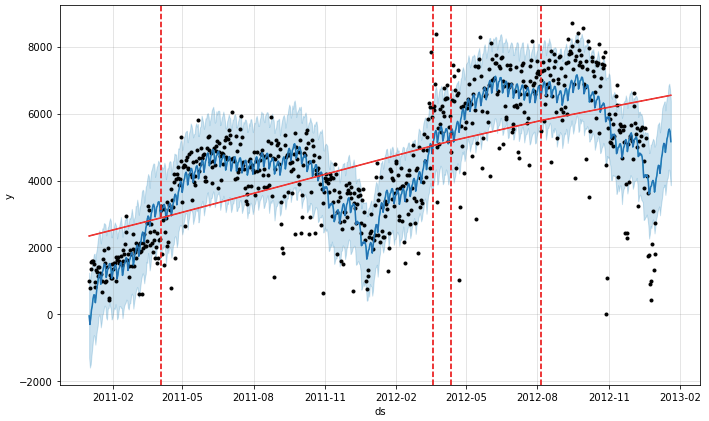
The simple code below shows how you can build a very reasonable model using the default setting. I also generate 20 data points and forecasts for future periods. The output graph shows the trend, the tolerance band, and the dashed lines that partitions the time series into several time windows. It is easy to identify the anomalies in the graph.
future= bike_model_0.make_future_dataframe(periods=20, freq='d')
future.tail()

bike_model_0_data=bike_model_0.predict(future)
bike_model_0_data.tail()

from prophet.plot import add_changepoints_to_plot
forecast = bike_model_0.fit(bike).predict(future)
fig= bike_model_0.plot(forecast)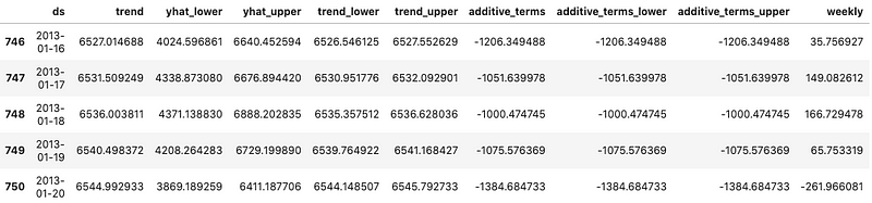
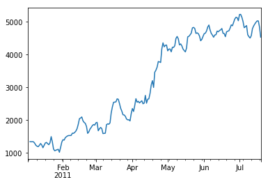
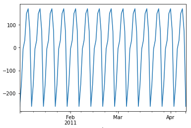
We can examine the “trend”, the “weekly” pattern, and the “monthly” pattern:
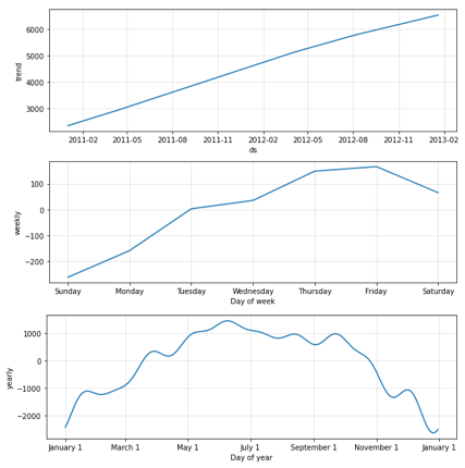
You can modify the default model with your domain knowledge for your particular time series. The trend component can be a connected piecewise line with many change points. The syntax Prophet() allows a large number of (up to 29) potential change points. But what if we specify too many segments that result in overfitting? The algorithm uses L1 regularization to keep the change points as few as possible. for more discussions, click “Business Forecasting with Facebook’s ‘Prophet’”.
(3.1) Diagnostics
# Python
from prophet.diagnostics import cross_validation
bike_0_cv = cross_validation(bike_model_0,
                         initial='100 days',
                         period='180 days',
                         horizon = '365 days')
bike_0_cv.head()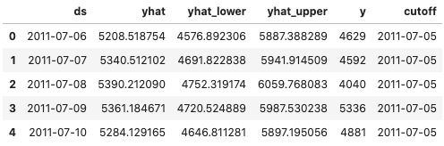
# Python
from prophet.diagnostics import performance_metrics
bike_0_p = performance_metrics(bike_0_cv)
bike_0_p.head()
The GAM is a powerful machine learning technique, though it does not receive sufficient popularity like random forest or gradient boosting in the data science community. It was originally invented by Trevor Hastie and Robert Tibshirani in 1986. You can find more detail on GAM in “Explain Your Model with Microsoft’s InterpretML”.
(5) RNN/LSTM/GRU
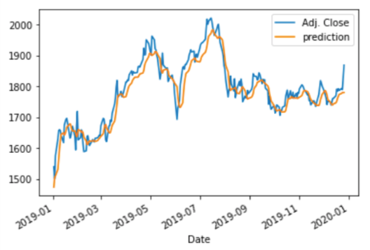
Stock price time series do not follow fixed patterns like business time series. Finding anomalies in a stock price time series has many applications and trading strategies, as detailed in “Algorithmic Trading with Technical Indicators in R”, or “Stock Market Anomalies” and “Stock Market Anomaly Detection” Are Two Different Things.
As said before, anomaly detection is about forming the norm to reveal the anomalies. The Recursive Neural Network (RNN), Long Short-Term Model (LSTM), and Gated recurrent unit (GRU) are deep learning methods that provide great predictability. With the predicted values, you can define anomalies as one to three standard deviations from the predicted values, or any reasonable stylized definitions. For the prediction technique, please read “A Technical Guide on RNN/LSTM/GRU for Stock Price Prediction” which provides great detail in modeling and programming.
Free Time Series Datasets
For readers who are looking for a dataset to practice time series anomaly detection, I list a few free time series datasets in this section. These sample datasets can be decomposed by seasonal-trend decomposition.
- Residential Power Usage: This data set contains hourly power usage in kWh starting from 01–06–2016 to August 2020. The dataset has marked notes for weekdays, weekends, COVID lockdown & vacation days in the notes category column.
- Electricity Power Monthly: You can search for “the U.S. monthly electricity power” from 2008 to 2010 by the state on this website.
- Hourly Energy Consumption: This dataset has over 10 years of hourly energy consumption data in Megawatts.
- Electricity: This dataset contains 45,312 instances from 1996–05–07 to 1998–12–05. Each example of the dataset refers to a period of 30 minutes, i.e. there are 48 instances for each period of one day. Each example on the dataset has 5 fields, the day of the week, the time stamp, the New South Wales electricity demand, the Victoria electricity demand, the scheduled electricity transfer between states, and the class label.
- Smart meter data: This dataset contains the energy consumption readings for a sample of 5,567 London Households that took part in the UK Power Networks-led Low Carbon London project between November 2011 and February 2014.
Conclusion
I hope this article gives you a better understanding of this topic. If you like to have a comprehensive review, the following sequence will help:
- Part 1: “Anomaly Detection for Time Series“
- Part 2: “Detecting the Change Points in a Time Series”
- Part 3: “Algorithmic Trading with Technical Indicators in R”
- Part 4: “Kalman Filter Explained!”
- Part 5: “Business Forecasting with Facebook’s “Prophet”
- Part 6: “Time Series with Zillow’s Luminaire — Part I Data Exploration”
- Part 7: “Time Series with Zillow’s Luminaire — Part II Optimal Specifications”
- Part 8: “Time Series with Zillow’s Luminaire — Part III Modeling”
- Part 9: “A Technical Guide on RNN/LSTM/GRU for Stock Price Prediction”
Readers are recommended to purchase the books by Chris Kuo:

- The Handbook of NLP with Gensim: https://a.co/d/08ciyih
- The explainable AI: https://a.co/d/cNL8Hu4
- Transfer learning for image classification: https://a.co/d/hLdCkMH
- Modern time series anomaly detection: https://a.co/d/ieIbAxM
- Handbook of Anomaly Detection: https://a.co/d/5sKS8bI


