Practical algorithmic trading — (1) Why algo trading and technical indicators?

Everyday there are millions of data analysts, data scientists, data engineers, or quants who analyze various financial factors for their investment decisions. Algorithmic trading, the use of computer algorithms to automate the process of buying and selling financial securities in the markets, is the major channel of investment in today’s economy. In this “practical algorithmic trading” series, I will introduce free Python tools including visualization, technical indicators, backtesting, and evaluation metrics.

Algorithmic trading is also called algo trading or automated trading. The algorithms are pre-researched rules that instruct when and how trades are executed based on various market data and conditions. These algorithms are viewed as the secret source of profitable trades. Algorithmic trading involves extensive data analysis for price movements, trading volume, technical indicators, and fundamental data.

Trading around the world

The world stock markets operate in all the time zones unceasingly. Let’s travel around the world to see the major stock exchanges. Our flight starts with the Wellington Stock Exchange in New Zealand (GMT+13), then the Sydney Stock Exchange in Australia (GMT+11), then the Tokyo Stock Exchange in Japan (GMT+9), then the Shanghai Stock Exchange in China (GMT+8), then the Mumbai Stock Exchange in India (GMT+5:30), then the Dubai Financial Market in the United Arab Emirates (GMT+4) and the Moscow Exchange in Moscow, Russia (GMT+4), then the Frankfurt Stock Exchange in Germany (GMT+1), then the London Stock Exchange in the United Kingdom (GMT+0), then the New York Stock Exchange in the United States (GMT-5) and the Toronto Stock Exchange in Canada (GMT-5). Which time zones do you do your trading?

Information can travels fast across different time zones. Before an exchange rings the bell, people already post tweets or share news with people in other time zones. Arbitrage trading opportunities exist across multiple time zones. This is one example of algo trading.

Who do algorithmic trading?

Let’s see a few types of investors who do algorithmic trading. The first type is individual traders. There are millions of active individual traders around the world analyzing and executing their trades. Are you a quantitative analyst? Quantitative analysts and researchers are interested in algorithmic trading as they develop and test trading models, strategies, and algorithms. Many of them come from a quantitative background since high school. They utilize mathematical and statistical techniques to identify patterns, create trading signals, and optimize trading algorithms.

Institutional Investors such as hedge funds, asset management firms, and pension funds, are the serious algorithmic traders. They manage large portfolios and may utilize algorithmic trading to execute trades efficiently, manage risk, and enhance returns. Market makers are algorithmic traders too. Market makers play a crucial role in maintaining liquidity. They provide bid and ask prices for any securities with the intention of buying from sellers and selling to buyers. They essentially act as intermediaries between buyers and sellers, ensuring that there is a continuous flow of trading activity. Finally, FinTech companies use algorithmic trading too. They develop algorithmic trading software and services to traders and financial institutions.

What are the advantages of algorithmic trading?

Algorithmic trading automatically generates and executes buy or sell orders. It can execute trades at a much faster pace than manual trading and can lead to better trade execution and increased profitability. Some institutional traders operates high-frequency trading that analyzing market data, identifying opportunities, and executing trades in milliseconds.

Algorithmic trading provides the ability to process large amounts of data including multiple indicators, news feeds, and historical prices, to identify trading opportunities. This ability to process and interpret large data sets quickly can lead to more informed and data-driven trading decisions. While institutional investors certainly can process large amounts of data, this advantage is especially appealing to retail investors who can conduct analysis on vast amount of data in a platform.

Great. Let’s start the first step by learning whether to download financial data for free. The Jupyter notebook is available via this link.

Free download for the stock market data

The yfinance library is a popular Python library that allows users to easily retrieve historical price data, financial statements, and other essential financial information. Below is the sample code to download “QQQ” daily historical data.

! pip install yfinance
import numpy as np
import pandas as pd
import yfinance as yf
import matplotlib.pyplot as plt

# Retrieve historical stock price data for QQQ
qqq = yf.Ticker("QQQ")
data = qqq.history(start="2021-01-01", end="2023-12-31")
data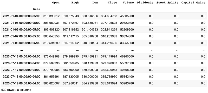

Is yfinance free? Yes, it is. You can even download granular data like 1min/2min/5min, called tick data. But yfinance only offers tick data for 7 days. If you need historical tick data for a long period, you will need to order from tick data providers.

Free download for the cryptocurrency data

Other than stock market data, here let’s learn how to download cryptocurrency data. The cryptocmd library offers free historical cryptocurrency data from CoinMarketCap. You can pip install this library through this pypi page. As of today, the top five cryptocurrencies are Bitcoin (“BTC”), Ethereum (“ETH”), Tether USD (“USDT”), Ripple (”XRP”), and Binance Coin “BNB”. Below I download the data for “XRP”. All these data downloads have the same data format like “Date”, “Open”, “High”, “Low”, “Close”, “Volume”. This enables easy programming.

! pip install cryptocmd

from cryptocmd import CmcScraper

# initialise scraper without time interval
scraper = CmcScraper("XRP")

# Pandas dataFrame for the same data
data = scraper.get_dataframe()
data

If you want to trade other commodities such as foreign exchange trading that buys one currency and sell another, you will need to set up a paid account with foreign exchange data vendors.

You may have seen that many trading platforms visualize financial market data. In this introductory post, let’s become familiar with plotting functions in Python.

Visualization for insights

Traders use various types of charts and graphs to gain insights into market trends, patterns, and potential opportunities. By visually observing price patterns, traders can identify trends, support and resistance levels, and potential price reversal points. Plotted charts enable traders to apply technical analysis methods effectively and make informed buy or sell decisions based on signals derived from the data. Plotting data allows traders to recognize common chart patterns, such as head and shoulders, double tops/bottoms, and flags. These patterns can serve as potential signals for entering or exiting trades.

Here let me introduce a lightweight, open source library called mplfinance. Its github has been starred by 3k users. You can install it by:

!pip install mplfinance

Let’s learn how to use it. While I introduce the tool, I will also provide the background knowledge.

Candle chart in yahoo style

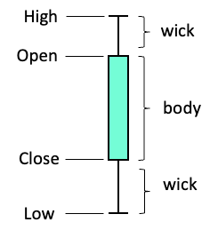
A candlestick chart shows the open, high, low, and close prices for a specific time period. Each candlestick represents the price action during that time frame. A candlestick has the body part and the wick part.

Body: The rectangular part represents the price range between the open and close prices. If the close price is higher than the open price, the body is typically filled with green color, indicating a bullish (positive) candlestick. Otherwise the body is red, indicating a bearish (negative) candlestick.
Wick: The thin lines extending from the top and bottom of the body are called wicks. They represent the price range between the high and low prices during the specified time period.

Let’s visualize candlesticks for “QQQ” in the past 30 days:

import mplfinance as mpf
days = -30
mpf.plot(data[days:], figratio=(12,4), type='candle', style="yahoo")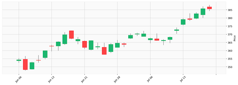

Line chart in yahoo style

Suppose you want to see the overall trend, a line chart is a good choice.

mpf.plot(data[days:], figratio=(12,4), type='line', style="yahoo")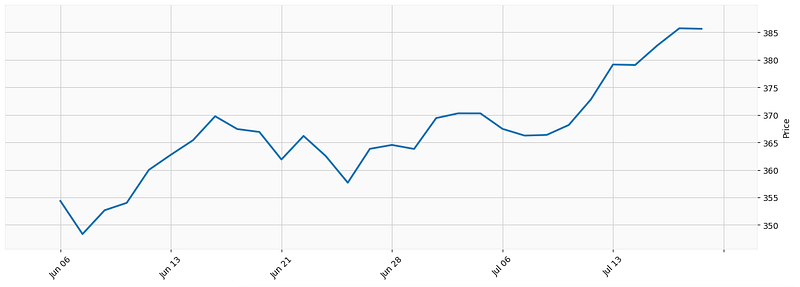

Renko chart

A Renko chart is a type of financial chart to visualize price movements in a simplified manner. It is named after the Japanese word “renga,” which means “brick,” as the chart consists of bricks or blocks that represent price movements. Unlike traditional price charts like line charts, bar charts, or candlestick charts that based on time intervals, Renko charts focus solely on price movement. Renko charts help filter out market noise and focus on the underlying price trend. Traders and technical analysts use Renko charts to identify trends, support and resistance levels, and potential entry or exit points for trading strategies.

Renko charts have two main types of bricks: bullish (typically colored white or green) and bearish (usually colored black or red). If the price moves upward and surpasses the top of the previous brick by at least the brick size, a new bullish brick is added above the previous one. Conversely, if the price moves downward and falls below the bottom of the previous brick by the brick size, a new bearish brick is added below the previous one. Let’s plot it now.

days = -300
mpf.plot(data[days:], figratio=(12,4), type='renko', style="yahoo")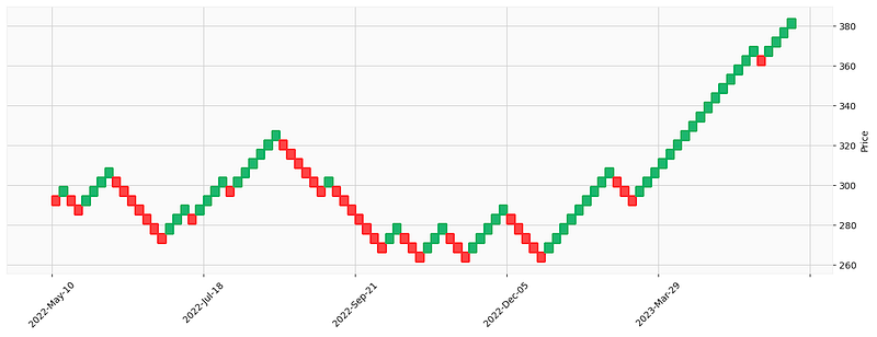

You can observe a long uptrend in recent days in the above renko chart. This helps traders to quick evaluate an uptrend or downtrend.

Candle chart with moving average lines

Suppose you like to add moving average lines to the candlesticks, you can do the following:

days = -50
mpf.plot(data[days:], figratio=(12,4), type='candle', style="yahoo", mav=(5,10,15))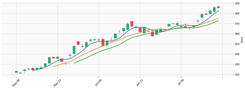

How about volume? Yes. You can add volume too.

Candle chart with moving average lines and volume

Let’s include volume in the code.

mpf.plot(data[days:], figratio=(12,4), type='candle', style="yahoo", mav=(5,10,15),volume=True)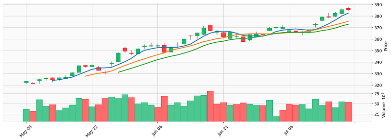

The above chart excluding non-trading days like Saturday, Sunday or holidays. Sometimes it is helpful to include non-trading days.

Candle chart with non-trading days

Suppose you also want to show the non-trading days, you can do:

mpf.plot(data[days:], figratio=(12,4), type='candle', style="yahoo", mav=(5,10,15),volume=True,show_nontrading=True)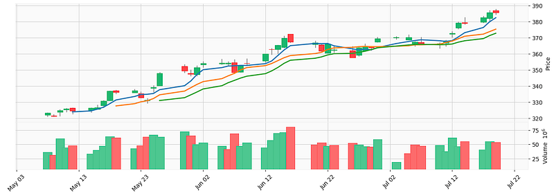

Knowing how to plot the data, let’s learn what technical indicators are, and some of the popular technical indicators.

Popular technical indicators

Technical indicators are mathematical formulas used in technical analysis. They are based on historical price data and are used to identify patterns and trends in the market. Technical indicators are lagging indicators. Strictly speaking they cannot forecast future price movements. But some price trends can be foreseen. Technical indicators can help to get insights into future price movements. Traders use them to form buy and sell strategies, to find the key levels of support and resistance, and to set stop loss levels.

One of the most popular open source Python library for technical analysis is ta-lib (Technical Analysis Library). Let’s get to know this library, and then let’s learn a few common technical indicators introduce Moving Averages (MA), Relative Strength Index (RSI), and Bollinger Bands (BB).

Install TA-lib

The TA-Lib library has more than 150 technical indicators. It is widely used by software developers and quants to perform technical analysis. This open source Python library can be easily installed by doing the following:

pip install TA-Lib

If you use Google Colab, you will use curl which is a command-line tool for getting or sending data including files using URL syntax. Run the following code in a Jupyter notebook cell:

#!pip install TA-Lib
!curl -L http://prdownloads.sourceforge.net/ta-lib/ta-lib-0.4.0-src.tar.gz -O && tar xzvf ta-lib-0.4.0-src.tar.gz
!cd ta-lib && ./configure --prefix=/usr && make && make install && cd - && pip install ta-lib

Now let’s first learn moving averages.

Simple Moving Averages (SMA)

This indicator calculates the average price of a security over a specific time period. I generate a 5-day moving average and a 20-day moving average. The shorter term moving average is called the fast moving average and the longer term moving average is called the slow moving average. The syntax is talib.SMA(price, timeperiod).

import pandas as pd
import talib
data['SMA5'] = talib.SMA(data['Close'], timeperiod=5)
data['SMA20'] = talib.SMA(data['Close'], timeperiod=20)
#data.dropna(inplace=True)
data

Let’s plot the fast MA in blue and the slow MA in orange.

import mplfinance as mpf

days = -100

indicators = [
    mpf.make_addplot(data['SMA5'][days:], color='blue', width=1.5),
    mpf.make_addplot(data['SMA20'][days:], color='orange', width=1.5),
]

mpf.plot(data[days:], figratio=(12,4), type='candle', style="yahoo", volume=True, addplot=indicators)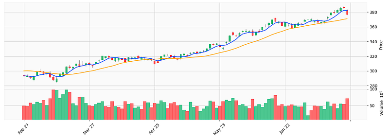

When the fast MA crosses to above the slow MA, it indicates a new uptrend so it is a buy signal.

Exponential Moving Averages (EMA)

EMAs are similar to SMAs, but they give more weight to recent price changes. Below let’s generate and plot the EMAs. Notice that I add the legend to the plot. The mplfinance library itself does not replicate the legend functions that the matplotlib library can produce.

data['EMA5'] = talib.EMA(data['Close'], timeperiod=5)
data['EMA20'] = talib.EMA(data['Close'], timeperiod=20)

import mplfinance as mpf
import matplotlib.pyplot as plt
style = mpf.make_mpf_style(marketcolors=mpf.make_marketcolors(up="g", down="r",inherit=True),
                           gridcolor="gray", gridstyle="--", gridaxis="both")
days = -100

added_plots = {"EMA5" : mpf.make_addplot(data['EMA5'].iloc[days:],width=1.5),
               "EMA20" : mpf.make_addplot(data['EMA20'].iloc[days:],width=1.5)
}
plt.figure(figsize=(10,20))
fig, axes = mpf.plot(data.iloc[days:, 0:5], type="candle", style=style,
                     addplot=list(added_plots.values()),
                     volume=True,
                     returnfig=True)
                     
axes[0].legend([None]*(len(added_plots)+2))
handles = axes[0].get_legend().legend_handles
axes[0].legend(handles=handles[2:],labels=list(added_plots.keys()))

axes[0].set_ylabel("Price")
axes[2].set_ylabel("Volume")

The code produces the price and volume sections.

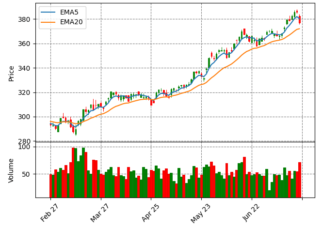
The 5-day EMA5 are closer to the price than the 20-day EMA20. This is expected because 5-day averages are more sensitive to price movement. Similiar to SMA, when the fast moving average crosses to above the slow moving average, it indicates a new uptrend so it is a buy signal.

Relative Strength Index (RSI)

Sometimes we want to understand if a stock is overbought or oversold. If it is oversold, the price can be too low that triggers a buy signal. And if it is overbought, the price can be too high and we should prepare to exit. The RSI indicator measures the magnitude of recent price changes to determine overbought or oversold conditions. It is calculated as the ratio of average gains to average losses over a specific time period. Let’s calculate RSI and plot it as a blue line.

# Retrieve historical stock price data for QQQ
qqq = yf.Ticker("QQQ")
data = qqq.history(start="2021-01-01", end="2023-12-31")

RSI_PERIOD = 14
data['rsi'] = talib.RSI(data['Close'], RSI_PERIOD)
data.tail(10)

# Plot it
import mplfinance as mpf

days = -50

indicators = [
    mpf.make_addplot(data['rsi'][days:], color='blue', width=1.5),
]

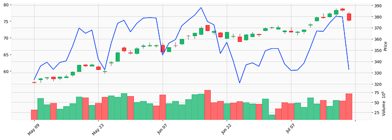
mpf.plot(data[days:], figratio=(12,4), type='candle', style="yahoo", volume=True, addplot=indicators)

RSI is a single line. When it is above a certain level, typically 70, it signals an overbought condition so it is a sell signal. When it is below a level, typically 30, it indicates an oversold condition so is a buy signal.

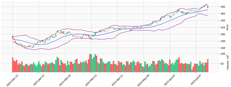
Bollinger Bands (BBANDS)

Bollinger Bands plot two standard deviations around a moving average to provide a visual representation of volatility. It can be used to identify breakouts and potential reversals in the market. The gap between the upper band and the lower band is called the Bollinger Bands.

It generates buy signals when the price falls below the lower band, indicating a potential oversold condition, and sell signals when the price rises above the upper band, indicating a potential overbought condition.

Let’s see the code:

# Retrieve historical stock price data for QQQ
qqq = yf.Ticker("QQQ")
data = qqq.history(start="2021-01-01", end="2023-12-31")

# Define the Bollinger Bands with 2-sd
data['upper_2sd'], data['mid_2sd'], data['lower_2sd'] = talib.BBANDS(data['Close'],
                                     nbdevup=2,
                                     nbdevdn=2,
                                     timeperiod=20)

# Plot
import mplfinance as mpf

days = -150

indicators = [
    mpf.make_addplot(data['upper_2sd'][days:], color='purple', width=1),
    mpf.make_addplot(data['mid_2sd'][days:], color='blue', width=1),
    mpf.make_addplot(data['lower_2sd'][days:], color='purple', width=1)
]

mpf.plot(data[days:], figratio=(12,4), type='candle', style="yahoo", volume=True, addplot=indicators)

It generates the following graph. You can observe there are times when the price touching the upper band, indicating a sell signal. Or the price touches the lower band, indicating a buy signal.

We will review more technical indicators in future posts.

All other technical indicators in TA-lib

At the time I am writing this post, there are 158 functions in TA-lib. You can print them out by running the following code.

import talib
# dict of functions by group
ta_func_grp = talib.get_function_groups()
ta_func_grp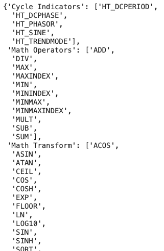

You can count the number of functions by group:

for key, value in ta_func_grp.items():
    print(key,":", len([item for item in value if item]))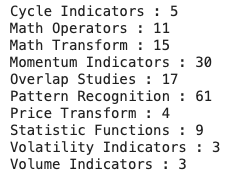

These group names are the conventional names by traders. For example, the “Cycle indicators” refer to indicators for cyclical patterns because most securities, especially futures, show a tendency for cyclical movements. Some traders may call them differently.

Summary

I hope this first chapter will give you an overview of algorithmic trading. In this post, we learn the very basic trading knowledge, the data library, the lightweight plotting library mplfinance. We also learned what technical indicators are, and a few technical indicators in the TA-lib library. You can download the Jupyter notebook via this link. In the next post, we will learn an important technique — Backtesting. We will how to backtest and optimize trading rules.

If you find this post helpful, please do not hesitate to contact with me or leave your feedback or Join Medium with my referral link — Chris Kuo/Dr. Dataman. If you are interested in algorithmic trading, you can take a look at