Practical Algorithmic Trading — (2) Backtesting

We may have a brilliant trading strategy, but without testing the strategy we are still not sure if it will work. Backtesting is the best sandbox for us to conduct testing, called paper trading. It applies a trading strategy to historical market data to determine how it would have performed in the past. This process is an important skill that quantitative analysts possess and implement frequently.

In this post, I will demonstrate how to use a popular open source libraries called backtesting.py for backtesting. I will also explain the common evaluate metrics. I then demonstrate two trading strategies in backtesting. After reading this post, you will be able to perform backtesting. You will also learn how to optimize your trading rules by different evaluation metrics to evaluate your trading styles. The Jupyter Notebook is available for download via this link.

Why do we need to do backtesting?

Backtesting is a crucial component of trading because it lets you to evaluate the performance of your trading strategies. By simulating trades using historical data, you can measure various performance metrics such as profit and loss, risk-adjusted returns, win rate, maximum drawdown, and other relevant statistics. This evaluation helps you determine whether a strategy has the potential to be profitable and if it aligns with their risk tolerance and financial goals.

Backtesting also let you optimize your trading strategies. For example, your strategy may be when the 10-day moving average crossing over the 30-day moving average. Why 10 or 30 days? Backtesting is your sandbox to test any number of days for the fast and slow moving average for a better outcome. This post will show you how to do backtesting, and the next post will show you how to search and optimize the parameters like here the number of days in a trading strategy.

Loss control is an important objective. Backtesting helps you assess the risks of your potential strategies to choose the ones that fit your trading style. This process enables traders to set realistic expectations, allocate capital appropriately, and implement risk mitigation strategies such as position sizing, stop-loss orders, and diversification.

Trading is subject to behavioral biases. Backtesting helps traders overcome behavioral biases that can affect decision-making. When traders rely solely on intuition or emotional judgment, they may be prone to biases such as hindsight bias or recency bias. Backtesting allows traders to make data-driven decisions based on historical evidence rather than relying on subjective perceptions or emotions.

I made Figure (A) for the roller coaster of emotion during 2019–2023 for many retail investors. The market was rosy in 2019 and arose the interest of many investors. Many investors tested the market by buying some stocks. The Covid Pandemic hit the market in March, 2020. He thought “I am glad not in the market”, and “even Warren Buffet sold all his Delta Airline stock”. So far so good. This investor has a small gain.

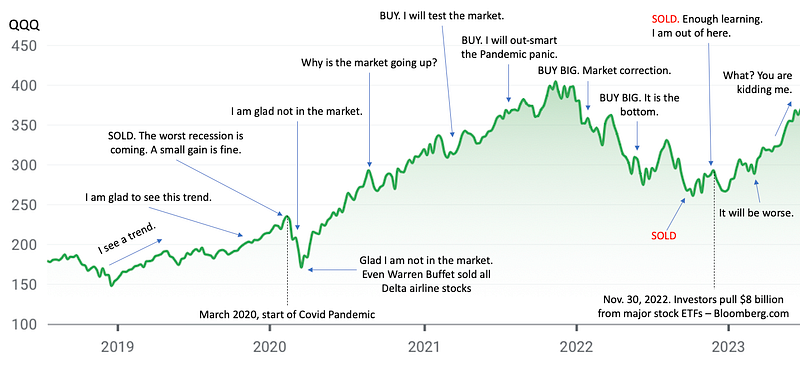
Who would predict the market could rise in 2021? Obviously the Fed’s policy was powerful. Seeing the uptrend in 2021, he thought to test the market again by buying some stocks. The uptrend happened only in 2021 and decreased in 2022. But in the beginning of 2022, he thought the uptrend should continue so he bought big. The market lost its momentum in 2022. He continued to buy because he attributed it to market correction. He almost bled to death in the third quarter of 2022 and got out of the market. According to Bloomberg.com, on Nov. 30, 2022 investors pull $8 billion from major stock ETFs. Then the market rose again in 2023. What can he say?

A key idea in backtesting

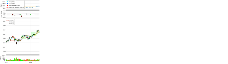
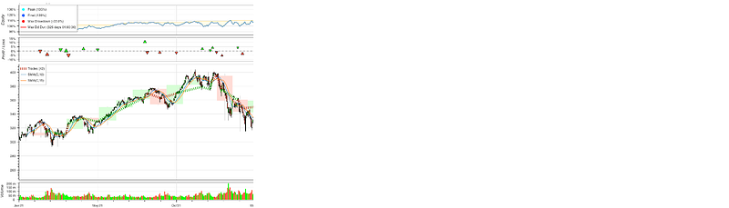
In backtesting, you are “going back to the history”. Any strategy should use data up to Day X in the past as I emphasize this idea in Figure (B), (C) and (D) for Day X1, X2, and X3. On Day X1, we only know information up to Day X1 and nothing after Day X1. The “buy” or “sell” signals are determined only use data up to X1. The same idea applies to any days like X2 or X3.

Hopefully now you agree with the need for backtesting, let’s continue to understand the tasks in backtesting.

What are the typical steps in Backtesting?

The common implementation includes the following tasks:

1. Load the data: Loading historical market data, such as price and volume, from various sources or file formats and converting it into a suitable format for analysis.
2. Strategy Implementation: Defining the rules and logic of a trading strategy, including indicators, entry and exit signals, and position management.
3. Trade Execution: Simulating the execution of trades based on the strategy’s rules, including managing position sizes, stop losses, and take-profit levels.
4. Performance Evaluation: Calculating various performance metrics, such as profitability, risk-adjusted returns, maximum drawdowns, and portfolio statistics, to assess the effectiveness of the strategy.
5. Visualization and Reporting: Generating charts, graphs, and summary reports to visualize the strategy’s performance and analyze its characteristics.

If you are looking for an open source and actively maintained Python libraries for backtesting, you may consider PyAlgoTrade, Backtrader, bt, and Backtesting.py. Each of them has its own style while carrying the common tasks. The reason that I adopt backtesting.py is its trading-like, sleek interface, and its evaluation metrics. In the following, I will first load the historical data and include the technical indicator library, then show you how to use the backtesting library. The Python notebook is available via this link.

Technical requirement

Now, let me introduce one popular open-source Python package for backtesting — backtesting.py. It is quite easy to pip install the library by doing:

pip3 install backtesting

We will also use the technical indicator ta-lib library to create simple moving average and exponential moving average. If you are running on your local environment, you can simple do:

!pip install TA-lib

If you use Google Colab, you will use curl which is a command-line tool for getting or sending data including files using URL syntax. Run the following code in a Jupyter notebook cell:

!curl -L http://prdownloads.sourceforge.net/ta-lib/ta-lib-0.4.0-src.tar.gz -O && tar xzvf ta-lib-0.4.0-src.tar.gz
!cd ta-lib && ./configure --prefix=/usr && make && make install && cd - && pip install ta-lib

We are ready to build our strategy and backtesting it.

Load the data

I will use yfinance, a very popular library stock market data library, to load the data. In this post, I will load daily data for symbol “QQQ” from 2021–01–01 to 2023–12–31. (at the time of this article, it is 2023–07–18).

import numpy as np
import pandas as pd
import yfinance as yf
qqq = yf.Ticker("QQQ")
data = qqq.history(start="2021-01-01", end="2023-12-31")
data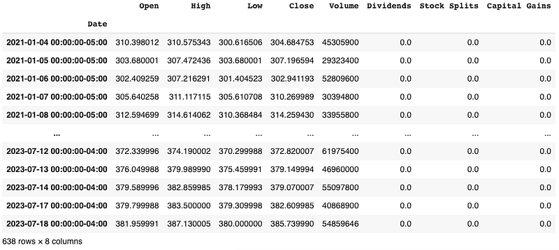

The yahoo stock historical data have the Open, High, Low, Close (often called OHLC), and Volume columns. These are the standard columns for most historical data libraries.

The code template

Below is the template to do backtesting with the backtesting.py library:

from backtesting import Backtest, Strategy
from backtesting.lib import crossover

class SmaCross(Strategy):

    def init(self):

    def next(self):

bt = Backtest(data, SmaCross,
              cash=10000, commission=.002,
              exclusive_orders=True)

output = bt.run()
bt.plot()

The template has the following fixed components:

• The placeholder for you to define your trading strategy: In this example, the class name is SmaCross(). It only has two functions init() and next(). The function init() does initilization and next() iterates through all data points.
• The Backtest() class to incorporate the data, the strategy, the cash, the commission cost.
• The code .run() to execute
• The code .plot() to plot.

These components will always be like that. So hopefully your learning curve will be quite flat. In next session, I will start to fill in the strategy. Notice that the class SmaCross(Strategy) inherits the class Strategy from backtesting. To understand what a Python class is, and what inheritance in object-orient programming does, you can take a look at the two articles:

• “Learning object-orient programming with Python in 10 minutes” for writing code in Python classes
• “Learning inheritance in object-oriented programming with Python” for class inheritance.

Define our own strategy

We will do the moving-average cross-over strategy. We call the class SmaCross() (you can call whatever you want). In the class, there will be two times series: the fast moving average and the slow moving average. The numbers of days for them are 10 and 20 days. We set them as the parameters sma_fast=10 for 10-day moving average and sma_slow=20 for 20-day moving average.

import talib
from backtesting import Backtest, Strategy
from backtesting.lib import crossover

class SmaCross(Strategy):
    sma_fast = 10
    sma_slow = 20

    def init(self):
        close = self.data['Close']
        self.sma1 = self.I(talib.SMA, close, self.sma_fast)
        self.sma2 = self.I(talib.SMA, close, self.sma_slow)

    def next(self):
        if crossover(self.sma1, self.sma2):
            self.buy()
        elif crossover(self.sma2, self.sma1):
            self.sell()

Now we define the fast and slow moving averages in the init() function. The init() will execute only one time. It defines the variable name self.sma1 and self.sma2 for the two moving averages.

The self.I() function is a blank function that lets you declare a technical indicator (“I” for indicator). The above code takes three inputs: the formula, the data, and the parameter for self.I(formula, data, parameter). It applies the formula talib.SMA to the data close with the parameter self.sma_fast to create an array of values self.sma1. You just need to remember “technical indicator” → “price data” → “parameter”.

The next() function performs backtesting by iterating through the past periods. The idea of backtesting is to go back to the past Day-X as if you only knew information up to Day-X and nothing after Day-X.

The function crossover(value1, value2) is a handy function defined by the library. It simply compares two values by checking if “value1>value2”. In our case, if the fast moving average self.sma1 is higher than the slow moving average self.sma2, then it is a “buy” and otherwise a “sell”.

That’s how you define a trading strategy in the class of this template. I will show you more examples in next few posts. Now let’s run the backtesting.

Run the backtesting

The Backtest(data, strategy, cash) takes at least three inputs: “data”, “strategy”, and “cash” for the initial cash value. Two more inputs in the following code are “commission” and “exclusive_orders”. The commission is the transaction fee. The “exclusive_orders” is set to “True” so a new order will auto-close the previous trade, making at most a single trade (long or short) in effect at each time.

bt = Backtest(data, SmaCross,
              cash=10000, commission=.002,
              exclusive_orders=True)

output = bt.run()
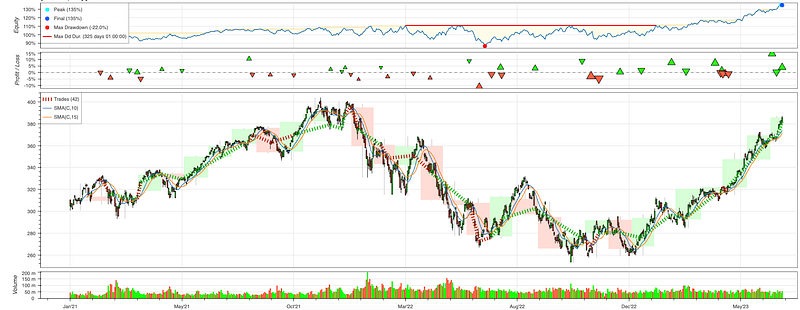
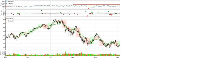
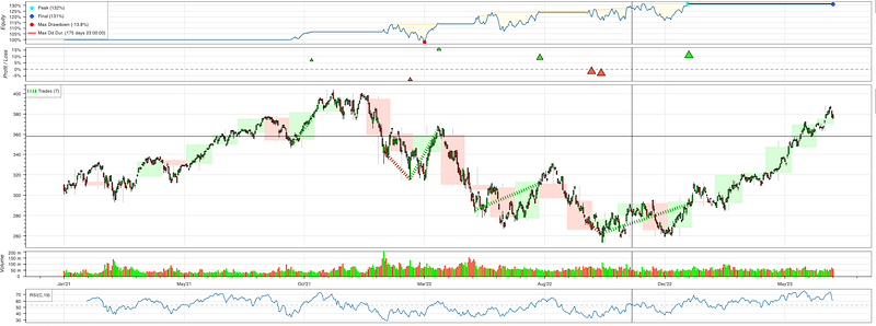
bt.plot()

You will like the trading dashboard as shown in Figure (E). It has four sections: “Equity”, “Profit/Loss”, “Trades” and “Volume”. When you point the cursor in the dashboard, it shows the horizontal and vertical lines to help you locate across the four sections.

Let me walk you through each section in the dashboard.

Equity

Figure (F) shows the equity section. It measures your earning in percentage. An 130% means your equity has 30% returns.

There is a legend in the left hand side, like Figure (G), showing the “peak”, the “final” of the equity. The “Max Drawdown” is an important term in trading. It is a peak-to-trouch decline during a specific period. For example, if a trading has $10k and the funds drop to $5k before coming back above $10k, then the trading account experienced a 50% drawdown.

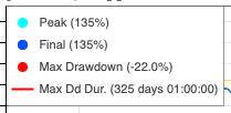
The “Max DD Dur.” is the maximum drawdown duration. It measures the longest time in the trading account that the drawdown has happened. The example shows 325 days with a red horizontal line, which means the longest time that the trading account has experienced a drawdown is 325 days. This is an important measure to a trader. During a drawdown period no one knows when the market will come back and how long the investor has to wait. Some investors may choose to close the trade.

Profit/Loss

The second sector is the Profit/Loss (PnL) section as shown in Figure (H). It has a dashed line in the middle for 0%. Above the dashed line are profitable results (showing in green triangle) and below it are unprofitable results (in red triangle).

Trades/volume

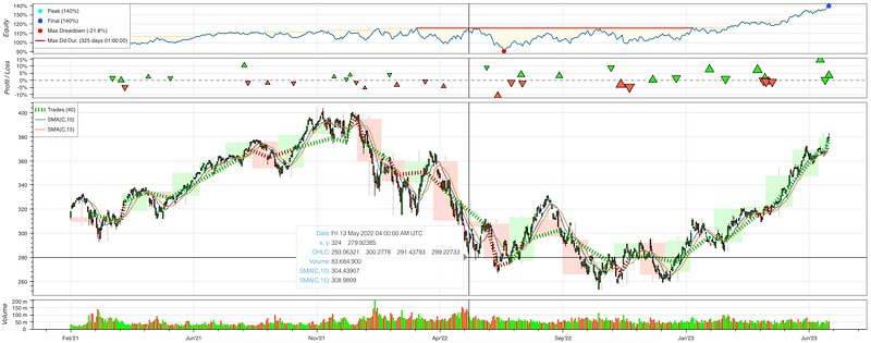
This is the largest section as shown in Figure (I). You can move the cursor to anywhere in the section to see the date of a particular date, the OHLC, the volume, and the indicators.

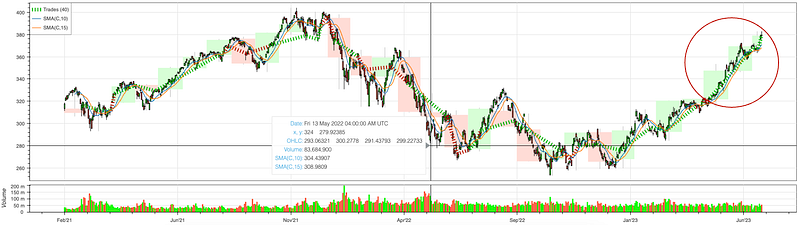
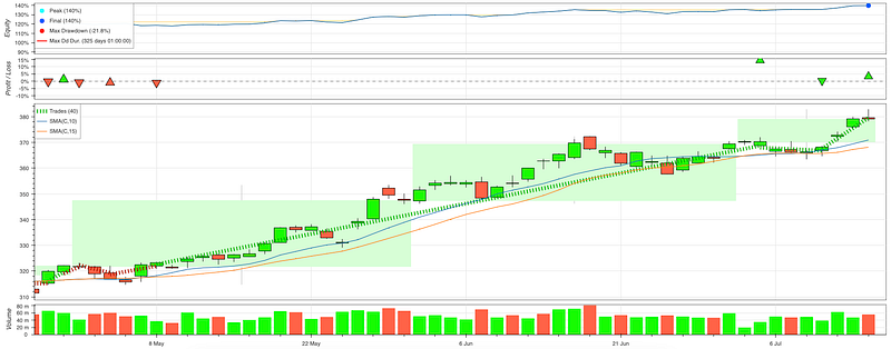
Let’s zoom in to the legend in Figure (I), as shown in Figure (J). The first one is the number of trades. In this examples there are 42 trades that end with negative returns, so the color is red.

The SMA(C,10) is the simple moving average for close price for 10 days. The SMA(C, 15) is 15 days.

Volume

The last section is the daily volume. Green bars mean positive daily returns and red bars mean negative returns.

Zoom in/Zoom out

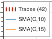
You can roll the scroll wheel of your mouse to zoom in and out of the dashboard. This is an extremely handy design. Figure (K) below shows the zoom-in view for the circled area in Figure (I). Notice there are three green boxes. Each box represents a month. If the close price in the end of a month is higher than the open price in the beginning of a month, the box is green. Otherwise the box can turn red.

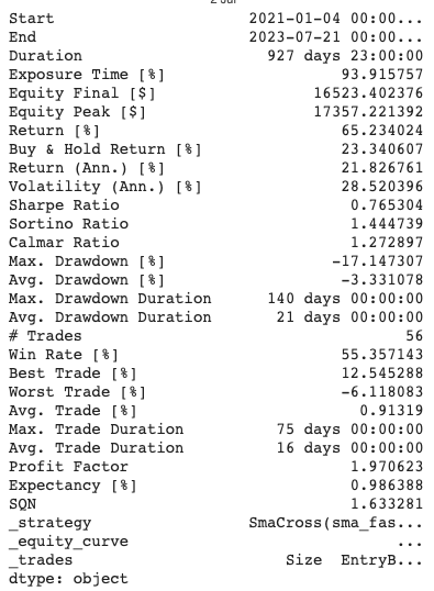
The evaluation metrics

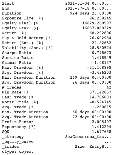
This library has the most common metrics that traders need to know. Figure (L) shows the metrics. I will explain one by one.

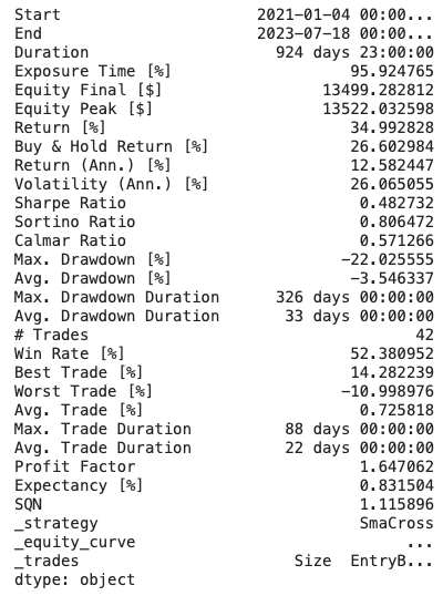
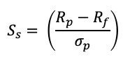
• start, End, Duration: the start and end dates and the duration between the start and end dates in the data.
• Exposure time (%): the percentage of days that the money is invested or “exposed” in the market.
• Equity final $ and Equity peak $: the final and the peak amounts of the equity.
• Return %: the percentage of returns of all the trades.
• Buy & hold return %: the return percentage if a trader just uses the buy-and-hold strategy that buys on the start date and sells on the end date.
• Return [Ann] %: The annualized return percentage.
• Volatility (Ann.) %: The annualized volatility. It is the standard deviation of daily return multiplied by the square root of 252, assuming there are 252 trading days in a given year.
• Sharpe ratio: The Sharpe ratio compares the return on an investment to the extra risk associated with it above and beyond a risk-free asset — the U.S. Treasury security. Figure (J) is the Sharpe ratio formula. It is the expected return Rp on the asset minuses the risk-free rate Rf, then divided by the standard deviation of daily return. The standard deviation measures volatility. A small standard deviation means there is not much volatility and is preferred. The lower the standard deviation, the less risk and the higher the Sharpe ratio. The (Rp — Rf) part of the formula is also called the market risk premium. It is the excess return above the risk-free rate.

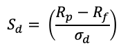
• Sortino ratio: The Sortino ratio is a variation of the Sharpe ratio as shown in Figure (K). It focuses on the volatility by using the asset’s standard deviation of negative portfolio returns, which is also called the “downside deviation”. The ratio was named after Frank A. Sortino. The only difference between Figure (J) and (K) is the standard deviation.

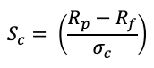
• Calmar ratio: The denominator is the maximum drawdown. It is -22% in Figure (I). A high Calmar ratio is desired.

Knowing the evaluation metrics, we will learn how to optimize the trading rules.

Optimize the trading rules

The 10-day and 20-day SMAs are trading rules. Why should they be 10 days or 20 days? Can we change them such that the target profit return % can be optimized? The answer is certainly yes. Another reason to optimize trading rules is the difference in the target metrics. The trading rules that pursue maximum profit return % will be different from the rules that pursue Sharpe ratio or Calmar ratio or other risk measures.

To optimize trading rules according to a specific target, you just need to use bt.optimize(). The above “SmaCross” class has two parameters: sma_fast =10 and sma_slow=20. The optimization can help to search for a range of values. Let’s say we want to test sma_fast to be anywhere between 2 days and 50 days, and sma_slow to be anywhere between 5 and 45 days. We can code them easily like below.

The constraint = is an optional function to impose the conditions. Suppose in our case we want sma_slow > sma_fast, it will only search for those parameters that meet the condition.

The maximize = function lets you specify any target metric in Figure (L). Here we assume the target metric is ‘Equity Final [$]’. Latter let’s test other target metrics. Then we are really to run it. This step will take a while due to its iterative process across all possible combinations.

stats = bt.optimize(
        sma_fast = range(2,50,1),
        sma_slow = range(5,45,1),
        constraint = lambda param: param.sma_slow > param.sma_fast,
        maximize='Equity Final [$]'
        )

bt.plot()
print(stats)

The outcome is in Figure (P). The “Return [%]” shows it can be 68.29% rather than the 34.99% in Figure (L).

Let’s give optimization one more try. This time let’s pursue the best Calmar ratio.

stats = bt.optimize(
        sma_fast = range(2,50,1),
        sma_slow = range(5,45,1),
        constraint = lambda param: param.sma_slow > param.sma_fast,
        maximize='Calmar Ratio'
        )

bt.plot()
print(stats)

The outcome is in Figure (Q). The Calmar ratio has improved to 1.27 if compared with 1.08 in Figure (P). The Calmar ratio is the excess returns divided by the maximum drawdown. A high Calmar ratio means the excess return % is good while the drawdown percentage is relatively small.

Relative Strength Index (RSI)

In the previous post we have introduced the RSI. This technical indicator helps us to understand if a stock is overbought or oversold. If it is oversold, the price can be too low that triggers a buy signal. And if it is overbought, the price can be too high and we should prepare to exit. The RSI indicator measures the magnitude of recent price changes to determine overbought or oversold conditions. It is calculated as the ratio of average gains to average losses over a specific time period.

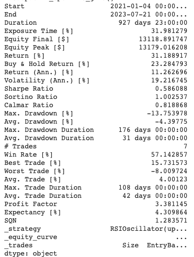
We can formulate a trading strategy by using RSI. When it is above 70, it signals an overbought condition so we will sell the asset. When it is below 30, we will buy the asset. Now let’s backtest the RSI strategy. The class RSIOscillator(Strategy) is our user-defined class. It sets the upper bound at 70 and lower bound at 30.

import numpy as np
import pandas as pd
import yfinance as yf
import matplotlib.pyplot as plt

# Retrieve historical stock price data for QQQ
qqq = yf.Ticker("QQQ")
data = qqq.history(start="2021-01-01", end="2023-12-23")
data

import talib
from backtesting import Backtest, Strategy
from backtesting.lib import crossover

class RSIOscillator(Strategy):

    upper_bound = 70
    lower_bound = 30
    rsi_window = 14

    def init(self):
        close = self.data['Close']
        self.rsi = self.I(talib.RSI, close, self.rsi_window)

    def next(self):

        if crossover(self.rsi, self.upper_bound):
          self.position.close()
        elif crossover(self.lower_bound, self.rsi):
          self.buy()

bt = Backtest(data, RSIOscillator,
              cash=10000, commission=.002,
              exclusive_orders=True)

We also perform optimization for the RSI trading rule. We will test a range of values for the upper bound, lower bound, and the RSI window. We set an obvious constraint that the upper bound should always be higher than the lower bound.

stats = bt.optimize(
    upper_bound = range(55,85,5),
    lower_bound = range(10, 45, 5),
    rsi_window = range(10, 30, 1),
    maximize = 'Equity Final [$]',
    constraint = lambda param: param.upper_bound > param.lower_bound
)
print(stats)
bt.plot()

The outcome shows the return % is 31.18%. In this case the active trading return % is higher than the buy & hold return 23.29%.

And we can check the dashboard. There is a fourth section in the bottom for RSI. When you move the cursor (not shown), it presents an horizontal line and a vertical line to help us locate the exact locations in these four sections.

Summary

In this post, we have learned the reasons for backtesting and the backtesting.py library to perform backtesting. We used the backtesting tool to evaluate the simple moving average and the RSI strategies. We have also learned how to optimize the trading strategies. You can download the Jupyter Notebook via this link.

If you find this post helpful, please do not hesitate to contact with me or leave your feedback or Join Medium with my referral link — Chris Kuo/Dr. Dataman. If you are interested in algorithmic trading, you can take a look at

• Practical algorithmic trading — (1) Why algo trading and technical indicators?
• Practical algorithmic trading — (2) Backtesting
• Reinforcement learning with human feedback (RLHF) for algorithmic trading
• “Algorithmic trading with technical indicators in R” or
• The book “Modern time series anomaly detection”.