Reinforcement Learning with Human Feedback (RLHF) for algorithmic trading

The success of ChatGPT brings the Reinforcement Learning with Human Feedback (RLHF) technique in the spotlight. RLHF is a type of machine learning approach that combines reinforcement learning (RL) and human feedback (HF) to improve the learning process. This post will give you a comprehensive understanding for RLHF. It describes RLHF applications in algorithmic trading (algo trading) and provides executable Python code examples. In the code examples, I will present a code example that does not have RLHF, then add RLHF to the code examples. I believe this is a natural way to learn a topic. I gradually take you deeper to the components in RLHF including Epsilon-greedy policy and Q-learning update rule. This will equip algorithmic traders for RLHF.

What is reinforce learning with human feedback?

It will be interesting to explain reinforcement learning with the classical game Pacman. The Pacman follows food and avoids ghosts in order to get higher scores. The food reinforces its actions every time its makes a move. In the traditional reinforcement learning (RL) terminology, the Pacman is the “agent” that learns from trial and error by interacting with an environment and receiving reward signals.

RL is like a carrot-and-stick rule that reinforces right actions to get more carrots and avoid punishments. Notice that this learning process of relying solely on environmental rewards and does not have human guidance. This can be problematic when the environment is more sophisticated and the agent can apparently make better choices with human feedback. RLHF incorporates the human feedback. This feedback can be in the forms of evaluations, rankings, or demonstrations from human experts.

Let’s write the RL and RLHF more formally.

The components of RF

Let’s think of the decision of the Packman in the game. It is an “agent” interacting with an “environment” to make the right “actions” for the maximize “reward”. This entire process can be modularized into components. Each component is actually a mathematical expression and can be programmed.

Agent: The Pacman.
Environment: The environment that the Pacman belongs to. It is the routes and the food and the ghosts.
State: The current condition of the environment at a particular time. Imagine that you take many snapshots of the Pacman moving in the environment. Every snapshot is a state.
Action: The decision made by the agent based on its current state. Because every snapshot is different, the agent has to make decisions accordingly. Life is like this, isn’t it?
Policy: This is the strategy for the action in a given state. This is like the overall principle. The policy of the Pacman is to “get more food and avoid the ghosts”. And the action is to move left or right in a state according to the policy.
Reward: The feedback signal for the Pacman based on its actions. The Pacman can take the right actions to maximize the reward over time.

The components of RLHF

Now I am making a more complex game. We are training an AI agent to play a basketball game. Suppose we like to see more slam dunks rather than bank shots. If it is just RL, we cannot provide our human feedback to improve the agent’s performance. But with RLHF we can add human feedback in the game. For those of you who do not play basketball, a slam duck is the player leaping into the air and slamming the ball into the net, yes, like Michael Jordan did. And a bank shot is to throw the ball to bounce off the backboard to go into the net. Let’s write RLHF more succinctly:

Initial RL: This is the same as RL. The agent starts learning by interacting with the game environment and receiving rewards based on its actions. It explores the game and gradually learns a policy that maximizes its cumulative rewards over time.
Human Feedback: Now we can provide human feedback to guide the agent’s actions. For example, we the experts can rank a slam dunk over a bank shot. So next time when the agent chooses to shoot, it can weigh a slam dunk more than a bank shot.
Reward Shaping: We can even provide feedback to modify the reward system. For example, rather than winning or losing the basketball game, we can offer more bonus points if there are more slam dunks in a game.
Iterative Improvement: Our feedback can be interactive. We can provide our feedback on the fly for the agent to learn from the combination of its own exploration, the game’s rewards, and the expert feedback.

By combining reinforcement learning with human feedback, the agent can learn more effectively and efficiently. The expert feedback helps the agent to avoid unnecessary exploration, learn faster, and improve its decision-making capabilities.

RLHF has many applications

RLHF has been utilized in many domains such as games, robotic design, autonomous vehicle system, and dialogue Systems.

RLHF is extremely successful in fine-tuning Large Language Models (LLMs) as we mentioned chatGPT earlier. When you see the generated texts by a LLM, you may find it still robotic or present harmful languages. This is where human feedback comes in. You can let it generate several similar answers and you provide your ranking feedback. Your ratings for the generated texts will be used as the data to fine-tune the LLM. The LLM will be able to choose the favorable texts because your feedback favor those choices. Human feedback also can prevent the generation of harmful or inappropriate content by an LLM. We just need to rate low for the problematic or biased responses. This helps the model to avoid such outputs in the future.

RLHF is also big in algorithmic trading. Let’s see how it works.

How is RLHF used in algorithmic trading?

Algorithmic trading uses computer algorithms to automatically execute trades based on a variety of factors, such as price, volume, or time. Many institutional and individual investors develop their own proprietary trading rules. Everyday there are billions of trading decisions dictated by algorithmic trading. The trading rules can continue to reinforce good decisions that result in positive gains. But the market isn’t so simple and if we let the trading system to execute on its own, the result can be detrimental. It is often the case that financial experts can foresee the coming of market turn-around and would like to interfere the automatic trading system. In this case, the expert feedback is important and can be incorporated. Let’s understand it more carefully:

Environment: This is the market including historical price data, relevant indicators, and other market factors.
State: This is the current market condition of the environment such as price, volume, or market information at a particular time.
Action: This is the trading action such as “buy” or “sell”.
Policy: This is the objective such as maximizing returns, minimizing risk, or achieving a specific target.
Reward: This is the gains in the market.
The reinforcement learning agent: Develop an agent that learns to make trading decisions based on the observed environment state. This agent can be implemented using algorithms such as Q-learning, Deep Q-Networks (DQN), or Proximal Policy Optimization (PPO). Of all these, Q-learning is the most popular. I will explain Q-learning, DQN, or PPO in the end of the post.

It’s important to note that incorporating human feedback in reinforcement learning for algorithmic trading is an ongoing research area, and the specific implementation can vary depending on the approach, algorithm, and feedback mechanism used. It requires careful consideration of the expertise and bias of human feedback, as well as potential limitations and challenges in real-world trading environments.

Let’s start with a stock example without RLHF

Below is a strategy that trades on “QQQ”. It uses market data from 2018–01–01 to 2022–12–31 to perform backtesting. Backtesting is an important method to evaluate an investment strategy. It applies your trading strategy to historical market data to test its results. It tells you how your trading strategy would have performed in the past and compares the results with actual market outcomes. The code notebook is available via this link.

import yfinance as yf
import numpy as np
import pandas as pd
import matplotlib.pyplot as plt

# Retrieve historical stock price data for QQQ from 2018 to 2022
qqq = yf.Ticker("QQQ")
data = qqq.history(start="2018-01-01", end="2022-12-31")

# Define the trading strategy
def trading_strategy(data):
    # Define your trading strategy based on the historical data
    # Example: Buy when the price is above the 50-day moving average, sell otherwise
    signals = pd.DataFrame(index=data.index)
    signals['Signal'] = np.where(data['Close'] > data['Close'].rolling(window=50).mean(), 1, 0)
    return signals

# Perform backtesting and calculate metrics
def backtest(data, signals):
    # Combine the historical data with the trading signals
    df = pd.concat([data, signals], axis=1).dropna()

    # Calculate daily returns
    df['Return'] = df['Close'].pct_change()

    # Calculate cumulative returns
    df['Cumulative Return'] = (1 + df['Return']).cumprod()

    # Calculate portfolio value
    df['Portfolio Value'] = df['Cumulative Return'] * initial_investment

    # Calculate metrics
    num_trading_days = len(df)
    returns = df['Return']
    cumulative_returns = df['Cumulative Return']
    variance = returns.var() * 252
    cvar = returns[returns <= np.percentile(returns, 5)].mean() * 252

    return df, cumulative_returns, variance, cvar

# Define initial investment amount
initial_investment = 10000

# Perform the trading strategy
signals = trading_strategy(data)

# Perform backtesting and calculate metrics
backtest_results, cumulative_returns, variance, cvar = backtest(data, signals)

# Plot the cumulative returns with entry and exit points
plt.figure(figsize=(10, 6))
plt.plot(backtest_results.index, cumulative_returns, label='Cumulative Returns')
plt.scatter(backtest_results[backtest_results['Signal'] == 1].index, backtest_results[backtest_results['Signal'] == 1]['Cumulative Return'], color='green', label='Buy')
plt.scatter(backtest_results[backtest_results['Signal'] == 0].index, backtest_results[backtest_results['Signal'] == 0]['Cumulative Return'], color='red', label='Sell')
plt.title('Cumulative Returns with Entry and Exit Points')
plt.xlabel('Date')
plt.ylabel('Cumulative Return')
plt.legend()
plt.grid(True)
plt.show()

# Print the calculated metrics
sharpe_ratio = (cumulative_returns[-1] - 1) / np.sqrt(variance)
cagr = (cumulative_returns[-1]) ** (252/len(data)) - 1

print(f"Sharpe Ratio: {sharpe_ratio:.2f}")
print(f"CAGR: {cagr:.2%}")
print(f"Cumulative Returns: {cumulative_returns[-1]:.2%}")
print(f"Variance: {variance:.6f}")
print(f"CVaR: {cvar:.6f}")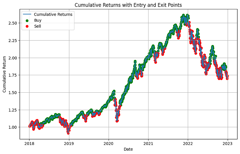

Its performance metrics are:

Sharpe Ratio: 2.82
CAGR: 11.71%
Cumulative Returns: 173.90%
Variance: 0.068559

In this example, we use the yfinance library to retrieve historical daily stock price data for the QQQ ETF. We implement a basic trading strategy. It buys when the price is above the 50-day moving average, and sells otherwise. You can instruct your own trading strategies.

To simulate trading, we calculate the positions based on the changes in the signal (Signal column). A positive value indicates a buy position, a negative value indicates a sell position, and 0 indicates no position. We accumulate the positions in the Position column. Finally, we visualize the stock price, moving averages, and the buy and sell signals using Matplotlib.

If you are new to algorithmic trading, here let me explain the common evaluation metrics.

CAGR stands for Compound Annual Growth Rate. It is a measure of the average annual growth rate of an investment over a given period of time. For example, if you invest $1000 in a stock that has a 10% CAGR, your investment will grow to $1100 after one year, $1210 after two years, and so on.
The Sharpe ratio is a measure of risk-adjusted return. It is calculated by dividing the excess return of an investment over a benchmark by the standard deviation of that excess return. For example, if an investment has a 10% return and a standard deviation of 5%, the Sharpe ratio would be 2. This means that the investment has a higher return than the benchmark, but with a lower level of risk. The Sharpe ratio is calculated as (R_a-R_b)/σ_a, where R_a is the expected return on the asset, R_b is the return on the risk-free asset, and σ_a is the standard deviation of the asset’s returns

This trading strategy does not receive human feedback. Now let’s add human feedback to it.

RLHF Code example 1

The following is an executable code example. Let’s read the lines.

import yfinance as yf
import pandas as pd
import numpy as np
import random

init_portfolio = 10000
 
# Retrieve historical stock price data for QQQ
qqq = yf.Ticker("QQQ")
data = qqq.history(start="2018-01-01", end="2022-12-31")

# Define the human feedback (example)
n = random.randint(0,len(data))
randomlist = []
for i in range(0,len(data)):
    n = random.randint(0,1)
    randomlist.append(n)
human_feedback = pd.DataFrame(index=data.index)
human_feedback['Feedback'] = randomlist  # 1 indicates positive feedback, 0 indicates negative feedback

# Define the trading strategy
def trading_strategy(data):
    # Define your trading strategy based on the historical data
    # Example: Buy when the price is above the 50-day moving average, sell otherwise
    signals = pd.DataFrame(index=data.index)
    signals['Signal'] = np.where(data['Close'] > data['Close'].rolling(window=50).mean(), 1, 0)
    return signals

# Apply reinforcement learning with human feedback
def reinforce_learning_with_human_feedback(data, human_feedback):
    signals = trading_strategy(data)  # Get initial signals from the trading strategy
    signals['Feedback'] = human_feedback['Feedback']  # Incorporate human feedback into signals

    # Iterate over the signals and adjust them based on human feedback
    for i in range(1, len(signals)):
        if signals['Feedback'].iloc[i] == 1 and signals['Signal'].iloc[i] == 0:
            signals['Signal'].iloc[i] = 1  # Adjust the signal to buy based on positive feedback
        elif signals['Feedback'].iloc[i] == 0 and signals['Signal'].iloc[i] == 1:
            signals['Signal'].iloc[i] = 0  # Adjust the signal to sell based on negative feedback
        
    return signals

# Perform trading with reinforcement learning and human feedback
trading_signals = reinforce_learning_with_human_feedback(data, human_feedback)

# Place trades based on recommended entry and exit points
def place_trades(data, signals):
    portfolio = init_portfolio  # Initialize portfolio

    # Iterate over the signals and place trades accordingly
    for i in range(1, len(signals)):
        if signals['Signal'].iloc[i] == 1 and signals['Signal'].iloc[i-1] == 0:
            # Buy QQQ
            price = data['Close'].iloc[i]
            shares = portfolio / price  # Invest entire portfolio in QQQ
            portfolio = 0  # Reset portfolio to 0
              
        elif signals['Signal'].iloc[i] == 0 and signals['Signal'].iloc[i-1] == 1:
            # Sell QQQ
            price = data['Close'].iloc[i]
            portfolio = shares * price  # Update portfolio value

    return portfolio

final_portfolio = place_trades(data, trading_signals)

# Print the final portfolio value
print(f"Final Portfolio Value: ${final_portfolio:.2f}")

The list human_feedback['Feedback'] has the values “1” for “like the trade” or “0” for “do not like the trade”. I set it as naïve random integers in this example. Obviously you want to replace it with a more intelligent human feedback.

The function trading_strategy() defines the action that buys when the price is above the 50-day moving average, and sells otherwise. You can replace with many other trading strategies.

The function reinforce_learning_with_human_feedback() get initial signals from the trading strategy in the list signals['Signal'] . It adds the human feedback human_feedback['Feedback'] . Then it adjust the initial trading signals with human feedback. It overwrites the signal “sell” if the human feedback is “buy”, and otherwise.

The function place_trades() calculates the number of shares and the portfolio based on the trading signals. This naïve human feedback yields the final portfolio value: $10477.77. You can re-run the code examples multiple times to see the final portfolio values.

To learn more on algorithmic trading and RLHF, Let me show you one more code example.

RLHF Code example 2

This time I will write the code in a Python class.

import numpy as np
import pandas as pd
import yfinance as yf

# Retrieve historical stock price data for QQQ
qqq = yf.Ticker("QQQ")
data = qqq.history(start="2018-01-01", end="2022-12-31")

# Define the Q-learning agent
class QLearningAgent:
    def __init__(self, num_states, num_actions, alpha, gamma):
        self.num_states = num_states
        self.num_actions = num_actions
        self.alpha = alpha  # Learning rate
        self.gamma = gamma  # Discount factor
        self.q_table = np.zeros((num_states, num_actions))

    def choose_action(self, state, epsilon):
        # Epsilon-greedy policy for action selection
        if np.random.uniform() < epsilon:
            return np.random.choice(self.num_actions)
        else:
            return np.argmax(self.q_table[state])

    def update_q_table(self, state, action, reward, next_state):
        # Q-learning update rule
        max_q_value = np.max(self.q_table[next_state])
        self.q_table[state, action] += self.alpha * (reward + self.gamma * max_q_value - self.q_table[state, action])

# Define the trading strategy with Q-learning and human feedback
def trading_strategy(data, q_agent, entry_points, exit_points, initial_investment):
    num_states = 2  # Number of states (0: out of the market, 1: in the market)
    num_actions = 2  # Number of actions (0: no trade, 1: trade)

    epsilon = 0.1  # Exploration rate
    total_reward = 0  # Track total reward
    portfolio_value = [initial_investment]  # Track portfolio value
    trades = []  # Track executed trades

    # Iterate over each trading day
    for i in range(len(data) - 1):
        state = 0 if portfolio_value[-1] == 0 else 1  # Current state

        # Check if an entry point exists for the current day
        if data.index[i] in entry_points:
            # Get the recommended action for the current day from human feedback
            action = entry_points[data.index[i]]

            # Execute the recommended action
            if action == 'BUY' and state == 0:
                state = 1  # Enter the market
                shares = portfolio_value[-1] / data['Close'][i]  # Buy as many shares as possible
                trades.append(('BUY', data.index[i], data['Close'][i], shares))
            elif action == 'SELL' and state == 1:
                state = 0  # Exit the market
                shares = portfolio_value[-1] / data['Close'][i]  # Sell all shares
                trades.append(('SELL', data.index[i], data['Close'][i], shares))

        # Calculate the reward based on the portfolio value change
        reward = (portfolio_value[-1] - portfolio_value[-2]) / portfolio_value[-2] if i > 0 else 0
        total_reward += reward

        # Choose the action using epsilon-greedy policy
        action = q_agent.choose_action(state, epsilon)

        # Execute the action
        if action == 1 and state == 0:
            state = 1  # Enter the market
            shares = portfolio_value[-1] / data['Close'][i]  # Buy as many shares as possible
            trades.append(('BUY', data.index[i], data['Close'][i], shares))
        elif action == 0 and state == 1:
            state = 0  # Exit the market
            shares = portfolio_value[-1] / data['Close'][i]  # Sell all shares
            trades.append(('SELL', data.index[i], data['Close'][i], shares))

        # Update the Q-table
        next_state = 0 if state == 0 else 1  # Next state
        q_agent.update_q_table(state, action, reward, next_state)

        # Update the portfolio value
        portfolio_value.append(shares * data['Close'][i])
        
    return total_reward, portfolio_value, trades

# Define the entry and exit points based on human feedback (example)
entry_points = {
    '2018-04-01': 'BUY',
    '2018-05-01': 'SELL',
    '2018-08-01': 'BUY',
    '2018-09-01': 'SELL'
}

exit_points = {
    '2018-05-01': 'SELL',
    '2018-06-01': 'BUY',
    '2018-09-01': 'SELL',
    '2018-10-01': 'BUY'
}

# Set the initial investment
initial_investment = 10000

# Create the Q-learning agent
q_agent = QLearningAgent(num_states=2, num_actions=2, alpha=0.2, gamma=0.9)

# Apply the trading strategy
total_reward, portfolio_value, trades = trading_strategy(data, q_agent, entry_points, exit_points, initial_investment)

# Calculate metrics
returns = np.diff(portfolio_value) / portfolio_value[:-1]
sharpe_ratio = np.sqrt(252) * np.mean(returns) / np.std(returns)
cagr = (portfolio_value[-1] / portfolio_value[0]) ** (252 / len(data)) - 1
cumulative_returns = (portfolio_value[-1] - portfolio_value[0]) / portfolio_value[0]
variance = np.var(returns)
cvar = np.mean(returns[returns < np.percentile(returns, 5)])
alpha, beta = np.polyfit(data['Close'].pct_change().dropna(), returns, deg=1)

# Plot portfolio performance
plt.figure(figsize=(10, 6))
plt.plot(data.index, portfolio_value, label='Portfolio Value')
plt.xlabel('Date')
plt.ylabel('Value')
plt.title('Portfolio Performance')
plt.legend()
plt.grid(True)
plt.show()

# Print metrics
print('Metrics:')
print(f'Sharpe Ratio: {sharpe_ratio:.3f}')
print(f'CAGR: {cagr:.3f}')
print(f'Cumulative Returns: {cumulative_returns:.3f}')
print(f'Variance: {variance:.6f}')
print(f'CVaR (Conditional Value at Risk): {cvar:.6f}')
print(f'Alpha: {alpha:.6f}')
print(f'Beta: {beta:.6f}')
print(f'portfolio_value: {portfolio_value[-1]:.6f}')

The class QLearningAgent() defines what the agent will do. In the code example, this agent only has two states: “1” for entering the market and “0” for exiting the market. The agent has two actions for either buying or selling the QQQ stock. It has the choose_action() function that describes its policy for action selection. Let me explain the “Epsilon-greedy policy”.

Epsilon-greedy policy is a reinforcement learning algorithm that uses a greedy approach to make decisions. It works by choosing the action that has the highest expected reward. The Epsilon-greedy policy is a simple and effective approach for solving many problems in reinforcement learning including robotics, game playing, and autonomous driving. It is simple and easy so it becomes popular. It is known that the main drawbacks is that it can be slow to converge to a solution, especially when the state space is large. Also, the Epsilon-greedy policy can sometimes lead to suboptimal solutions. But overall it is very acceptable.

Next, let me explain the Q-learning update rule. It is a rule used in Q-learning to update the Q-value of a state-action pair. The Q-value is a measure of the expected future reward that can be obtained by taking the action at the current state. The Q-value of a state-action pair can be updated by multiplying the current Q-value by a learning rate, and adding a negative exponential decay term. The learning rate controls the speed at which the Q-value updates, and the exponential decay term ensures that the Q-value decays over time. I will explain the Q-learning later.

Next, the function trading_strategy() defines when the human feedback is applied. It checks if an entry point exists for the current day, and then gets the recommended action from human feedback. It takes an action for “BUY” or “SELL” and recalculate the number of shares and portfolio value.

The human feedback in this example is very simple. It enters and exits the market on these specified days. Finally, it plots the portfolio performance as the following:

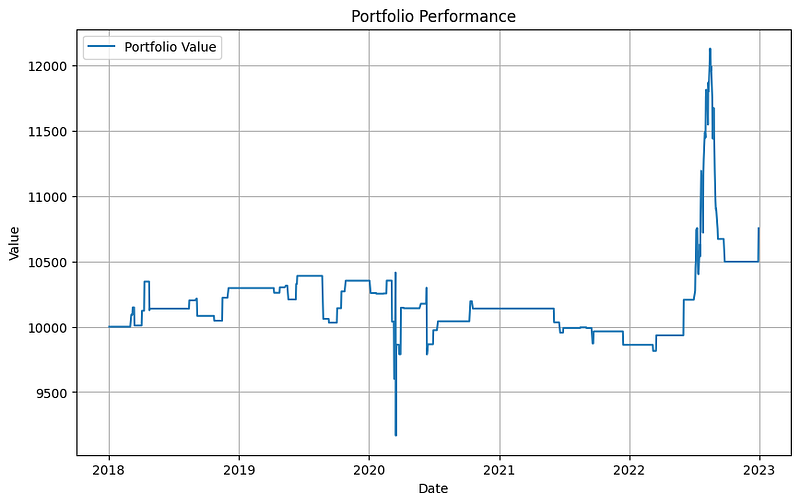
And the performance metrics are:

Sharpe Ratio: 0.194
CAGR: 0.015
Cumulative Returns: 0.075
Variance: 0.000042
CVaR (Conditional Value at Risk): -0.011010
Alpha: -0.052566
Beta: 0.000109
portfolio_value: 10753.106779

Now, I am going to explain what I left unexplained: Q-learning, Deep Q-Networks (DQN), Proximal Policy Optimization (PPO). Knowing them just make your knowledge for RLHF complete.

Summary

I trust this post can help your understanding on RLHF and its applications in algorithmic trading. If you find this post helpful, please do not hesitate to contact with me or leave your feedback or Join Medium with my referral link — Chris Kuo/Dr. Dataman.

If you are interested in algorithmic trading, you can take a look at

If you are interested in Large Language Models, you are highly recommended to take a look at:

I write the Q-learning, Deep Q-Networks (DQN), and the Proximal Policy Optimization (PPO) here in the Appendix so they will not overwhelm you. For most algorithmic traders, Q-learning is enough as shown in the above code example 2. But in case you want to dig deeper for further research.

Appendix: Q-learning

Q-learning is a popular reinforcement learning algorithm that enables an agent to learn an optimal policy in an environment without prior knowledge. It is a model-free, off-policy algorithm that uses a Q-value function to estimate the value of taking a certain action in a given state. In Q-learning, the goal of the agent is to maximize the cumulative reward over time. The Q-value represents the expected cumulative reward when taking a particular action in a given state. The Q-value function is updated iteratively based on the observed rewards and the agent’s estimates.

During the learning process, the agent explores the environment using an exploration-exploitation trade-off. It balances between exploring new actions and exploiting the current knowledge to maximize reward. The agent updates the Q-values using the Q-learning update rule, which incorporates the observed reward and the maximum expected future reward from the next state. The agent will learn the optimal policy that guides its actions.

Appendix: Deep Q-Networks (DQN)

Deep Q-Networks (DQN) extends Q-learning by combining reinforcement learning with deep neural networks. It was introduced by DeepMind in 2015 and has been successful in solving complex and high-dimensional reinforcement learning tasks.

The key idea behind DQN is to use a deep neural network, such as a convolutional neural network (CNN), to approximate the Q-value function. Instead of maintaining a Q-table, as in traditional Q-learning, the DQN agent learns to estimate Q-values directly from raw input observations. The DQN algorithm incorporates several techniques to stabilize and improve learning:

Experience Replay: DQN uses an experience replay buffer to store past experiences (state, action, reward, next state) observed during interactions with the environment. During training, mini-batches of experiences are sampled randomly from the buffer to break the correlation between consecutive experiences and improve learning efficiency.
Target Network: DQN employs a separate target network that provides the target Q-values during training. This target network has its parameters frozen for a certain number of iterations and then updated periodically to match the current Q-network. This stabilizes the learning process by providing more consistent target values.
Exploration vs. Exploitation: DQN balances exploration and exploitation using an epsilon-greedy strategy. Initially, the agent explores the environment by selecting random actions. As training progresses, it gradually reduces exploration and relies more on the learned policy for action selection.
Loss Function and Optimization: DQN minimizes the mean squared error loss between the predicted Q-values and the target Q-values. The optimization is performed using gradient descent algorithms, such as stochastic gradient descent (SGD) or variants like Adam.

DQN has demonstrated significant success in various challenging tasks, including playing Atari games, robotic control, and complex decision-making problems. It allows agents to learn directly from raw sensory inputs, enabling them to handle high-dimensional state spaces and make more sophisticated decisions.

Appendix: Proximal Policy Optimization (PPO)

What if there are many action choices? When the action spaces is continous, Proximal Policy Optimization (PPO) is a popular reinforcement learning algorithm. It was introduced by OpenAI in 2017 as an improvement over previous policy optimization methods.

PPO belongs to the family of policy gradient algorithms and aims to optimize a parameterized policy to maximize the expected cumulative reward. It works by iteratively collecting experience from the environment and updating the policy based on that experience.

The main idea behind PPO is to strike a balance between exploration and exploitation while ensuring stable policy updates. It achieves this through two key components: a surrogate objective function and a clipping mechanism.

The surrogate objective function in PPO compares the new policy’s probabilities of actions with the old policy’s probabilities. It constructs a surrogate objective that approximates the expected improvement in the policy. By maximizing this surrogate objective, PPO encourages policy updates that improve performance.

To ensure stability, PPO applies a clipping mechanism to the surrogate objective. Instead of allowing unrestricted policy updates, it limits the update to a range around the current policy. This clipping prevents large policy updates that can disrupt the learning process and helps maintain stability.

PPO also incorporates a form of importance sampling to adjust for the discrepancy between the new and old policies. This adjustment helps mitigate the issue of biased updates when using data collected from a different policy.

By iteratively collecting experience, calculating the surrogate objective, applying the clipping mechanism, and updating the policy, PPO learns an improved policy that maximizes the expected cumulative reward. It has been successfully applied to various reinforcement learning tasks, including robotics control, game playing, and simulated environments.