Explaining Your Model with Microsoft’s InterpretML

Model interpretability has become the main theme in the machine learning community. Many innovations have burgeoned. The InterpretML module, developed by a team in Microsoft Inc., offers prediction accuracy, and model interpretability, and aims at serving as a unified API. Its Github receives active updates. I have written a series of articles on model interpretability, including “Explain Your Model with the SHAP Values”, “Explain Any Models with the SHAP Values — Use the KernelExplainer”, “Explain Your Model with LIME”, “The SHAP with More Elegant Charts”, and “Creating Waterfall Plots for the SHAP Values for All Models”.

In this article, I am going to introduce a new method other than the SHAP. I will provide a gentle mathematical background and then show you how to interpret your model with InterpretML. If you want to do the hands-on practice first, You can jump to the modeling part, then come back to review the mathematical background.

The InterpretML Python Module

The InterpretML module was developed by a Microsoft team. The module leverages many libraries like Plotly, LIME, SHAP, and SALib, so is compatible with other modules. Based on the Generalized Additive Model (GAM) and GA2M algorithms, the Microsoft team developed an interpretability algorithm called the Explainable Boosting Machine (EBM). The development history is quite inspiring so I decided to briefly describe it.

Understand Generalized Additive Models

The Generalized Additive Models (GAMs) were invented by Trevor Hastie and Robert Tibshirani in 1986. The GAM is a powerful and yet simple technique, although it does not receive sufficient popularity like random forest or gradient boosting in the data science community. Let me highlight the idea of GAM:

• Relationships between the individual predictors and the dependent variable follow smooth patterns that can be linear or nonlinear. Figure (A) illustrates the relationship between x1 and y can be nonlinear.
• Additive: these smooth relationships can be estimated simultaneously and then added up.

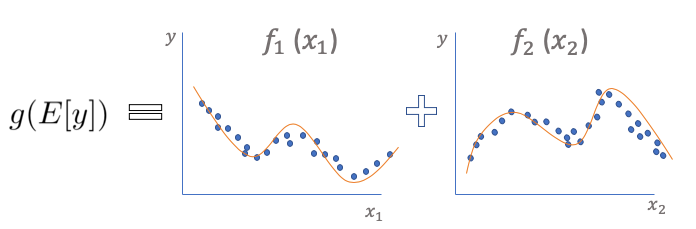
In Figure (A) the E(Y) denotes the expected value. The link function g() links the expected value to the predictor variables. The function f() is called the smooth or nonparametric function. (Nonparametric means that the shape of predictor functions is solely determined by the data. In contrast, parametric means the shape of predictor functions is defined by a certain function and parameters.) When the function f() becomes linear, GAM reduces to GLM. GLM is easy to interpret, and so is GAM.

If GAMs use smooth functions to fit data, will they fit too well by specifying high-degree smooth functions? How do Trevor Hastie and Robert Tibshirani 1986 overcome the overfitting challenge? They add an extra penalty to GAMs in the loss function for each smooth term. They also apply regularization techniques such as LASSO, Ridge, or Elastic Net. The case for GAMs includes:

• Easy to interpret.
• More flexible in fitting the data, and
• Regularizing the predictor functions to avoid overfitting.

It is worth mentioning that the GAM is also used in Facebook’s open-source “Prophet” module. See “Business Forecasting with Facebook’s Prophet”.

Add the Interaction Terms to GAM for Better Prediction Accuracy

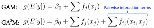
However, the predictability of GAMs is generally lower than more complex models that permit interactions. In the paper “Accurate Intelligible Models with Pairwise Interactions” by Lou et. al. (KDD-2013), they add interaction terms to the standard GAMs and call it GA2M — Generalized Additive Models plus Interactions. As a result, GA2M increases the prediction accuracy greatly but still preserves its nice interpretability.

The Explainability Boosting Machine (EBM)

The pairwise interaction terms in GA2M increase accuracy. However, it comes with another problem — it is extremely time-consuming and CPU-hungry. The Microsoft team proposed a solution called the Explainability Boosting Machine (EBM). The work is engineering. First, it trains each smooth function f() using machine learning techniques such as bagging and gradient boosting (that’s the name Boosting in EBM). Second, each feature is tested against all other features like a round-robin tournament. In a round-robin competition, each contestant meets every other contestant. In this way, the model finds the best feature function f() for each feature and shows how each feature contributes to the model’s prediction. Finally, EBM develops the GA2M algorithm in C++ and Python and takes advantage of joblib to provide multi-core and multi-machine parallelization.

InterpretML — A One-Stop Shop

I call it a one-stop shop because it has incorporated the key modeling tasks in a pipeline. These tasks include data exploration, model training, model performance comparison, and prediction interpretability at both the global and local levels. In the following code example, I am going to perform the tasks in (A) to (F):

• (A) Explore the Data
• (B) Train the Explainable Boosting Machine (EBM)
• (C) Performance: How Does the EBM Model Perform?
• (D) Global Interpretability — What the Model Says for All Data
• (E) Local Interpretability — What the Model Says for Individual Data
• (F) Dashboard: Put All in a Dashboard — This is the Best

First, do pip install -U interpret to install the module.

I will use the same red wine quality data so you can compare SHAP, LIME, and InterpretML, as I have been doing in “Explain Your Model with the SHAP Values”, “Explain Any Models with the SHAP Values — Use the KernelExplainer” or “Explain Your Model with LIME”. The target value of this dataset is the quality rating from low to high (0–10). The input variables are the content of each wine sample including fixed acidity, volatile acidity, citric acid, residual sugar, chlorides, free sulfur dioxide, total sulfur dioxide, density, pH, sulphates, and alcohol. There are 1,599 wine samples. The code is at the end of the article, or via this Github.

(A) Explore the Data

It presents a drop-down menu for the variables like Future (A). When you click the “Summary”, it presents the histogram of the target variable.

Choose the first variable “Fixed Acidity” in the drop-down menu. The Pearson Correlation of “Fixed Acidity” with the target variable is presented. After the correlation value, the histogram of “Fixed Acidity” is shown in blue color and the histogram of the target is in red. See Figure (E.1.2).

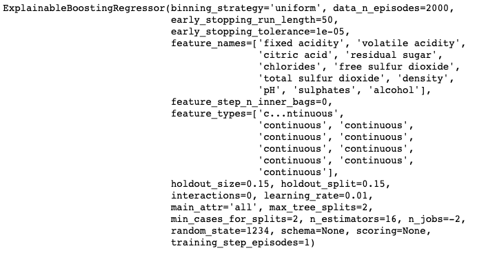
(B) Train the Explainable Boosting Machine (EBM)

Besides building the EBM model, I also build a linear regression and a regression tree model for comparison. The ExplainableBoostingREgressor() uses all the default hyper-parameters as shown in the output. You can specify any of the hyper-parameters.

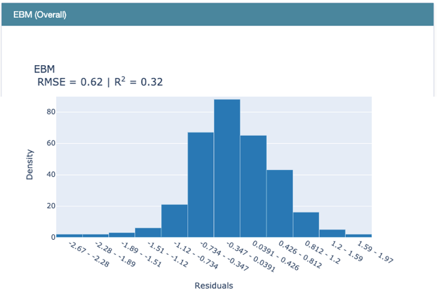
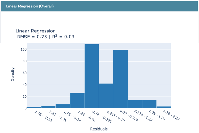
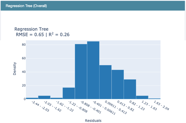
(C) How Does the EBM Model Perform?

Use RegressionPerf() to assess the performance of each model on the test data. Figure (E.3.1) shows the R-squared value of EBM is 0.32. Figure (E.3.1) and Figure (E.3.2) show the R-squared of the linear regression model is 0.03, and that of the regression tree is 0.26. So EBM shows stronger performance.

(D) Global Interpretability

The above code generates the EBM Overall in Figure (D.1). Choose “Summary” from the drop-down menu to show the overall variable importance. They are ranked in descending order with orange color.

Next, choose the first variable “Fixed Acidity” from the drop-down menu. Two plots show up: the Partial Dependent Plot (PDP) and the histogram of “Fixed Acidity”. The histogram indicates most of the values are between 6.0 to 10.0. The PDP presents the marginal effect of the feature on the predicted outcome of a machine learning model (J. H. Friedman 2001). It tells whether the relationship between the target and a feature is linear, monotonic, or more complex. In this example, the PDP shows there is a very mild linear and positive trend between “Fixed Acidity” and the target variable when “Fixed Acidity” is between 6.0 to 10.0.

(E) Local Interpretability

Let’s study the first five observations.

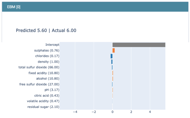
The drop-down menu lists the predicted value and the actual value for each record. See Figure (E.1). Let’s choose the first record.

Figure (E.2) shows the value of “Sulphates” is 0.76, and that of “Chlorides” is 0.17, and so on. The contributions of all variables for this record are ranked in descending order as below. “Sulphates” positively contribute to the target “quality”, while “Chlorides”, “Density”, etc. negatively contribute to the target. Because EBM is an additive model like GAM, the prediction is the sum of all the coefficients.

(F) Put All in a Dashboard

All of the above can be put together in a dashboard. Simply use a list to contain all the elements in the show() function:

The dashboard’s title is “Interpret ML Dashboard”. It has five tabs. The first tab “Overview” is an introductory page. The second tab “Data” presents the same plots as described above in the “(A) Explore the Data” section.

The “Data” Tab:

The “Performance” Tab:

The third tab “Performance” presents the same plots as described above in the “(C) How Does the EBM Model Perform” section.

The “Global” Tab:

The fourth tab “Global” presents the same plots as described above in the “(D) Global Interpretability” section.

The “Local” Tab:

The fifth tab “Local” presents the same plots as described above in the “(E) Local Interpretability” section.

For your convenience, I put all the code lines below. The code is also available via this Github.

If you find this article helpful, you can check other articles in the model explainability series:

Part I: Explain Your Model with the SHAP Values

Part II: The SHAP with More Elegant Charts

Part III: How Is the Partial Dependent Plot Calculated?

Part VI: An Explanation for eXplainable AI

Part V: Explain Any Models with the SHAP Values — Use the KernelExplainer

Part VI: The SHAP Values with H2O Models

Part VII: Explain Your Model with LIME

Part VIII: Explain Your Model with Microsoft’s InterpretML

Readers are recommended to purchase books by Chris Kuo:

• The explainable AI: https://a.co/d/cNL8Hu4
• Transfer learning for image classification: https://a.co/d/hLdCkMH
• Modern time series anomaly detection: https://a.co/d/ieIbAxM
• Handbook of Anomaly Detection: https://a.co/d/5sKS8bI