Explain Your Model with LIME

(Revised on June 16, 2022)

Why Is Model Interpretability so Important?

In this article, I will introduce the LIME approach. I will start with the questions that the inventors of LIME were concerned with, then walk you through their solutions. You may be interested in knowing their thought process or even adopting their problem-solving approach.

People typically agree that a linear model is more interpretable than a complicated machine learning model. Is it true? Do you think the following linear model is easily interpretable? Probably not. It has too many variables.

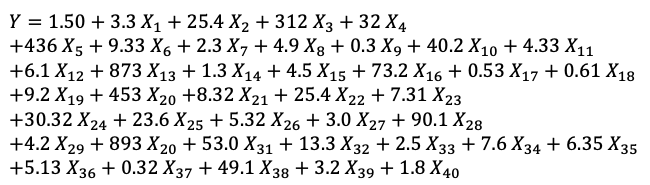
Besides the above concern, the second concern is that this model has many variables. For an individual prediction, only a few variables play significant roles in the prediction. The rest variables are almost irrelevant to an individual prediction.

These two questions are what Marco Tulio Ribeiro, Sameer Singh, and Carlos Guestrin, the authors of the paper “Why Should I Trust You?” Explaining the Predictions of Any Classifier (KDD2016), concerned about. Let’s see their augments.

(A) “Why Should I Trust You?”

The authors of LIME argue that we should build two types of trusts for a user to adopt a model:

• Trusting a prediction: a user will trust an individual prediction to act upon. No user wants to accept a model prediction on blind faith, especially if the consequences can be catastrophic.
• Trusting a model: the user gains enough trust that the model will behave in reasonable ways when deployed. Although in the modeling stage accuracy metrics (such as AUC — Area under the curve) is used on multiple validation datasets to mimic the real-world data, there often exist significant differences in the real-world data. Besides using the accuracy metrics, we need to test the individual prediction explanations.

(B) “Easily Interpretable” and “Local Fidelity”

They argue that a model should be easily interpretable. The linear equation in Figure (A) is probably not easily interpretable.

Second, for an individual prediction, there may be only a few variables influencing its predicted value. The interpretation should make sense from an individual prediction’s view. The authors of LIME call this local fidelity. Globally important features may not be important in the local context, and vice versa. Because of this, it could be the case that only a handful of variables directly relate to a local (individual) prediction, even if a model has hundreds of variables globally.

In summary, the authors of LIME have two criteria for model explainability:

• Easy to interpret: A linear model can have hundreds or thousands of variables. Is it more interpretable than a complex gradient boosting or deep learning model?
• Local fidelity: the explanation for individual predictions should at least be locally faithful, i.e. it must correspond to how the model behaves in the vicinity of the individual observation being predicted. The authors address that local fidelity does not imply global fidelity: globally important features may not be important in the local context, and vice versa. Because of this, it could be the case that only a handful of variables directly relate to a local (individual) prediction, even if a model has hundreds of variables globally.

That’s why they named their technique Local Interpretable Model-Agnostic Explanations (LIME) — It should be locally interpretable and able to explain any model.

(C) How Is LIME Different from SHAP?

In “Explain Your Model with the SHAP Values” I describe extensively how the SHAP (SHapley Additive exPlanations) is distinctly built on the Shapley value. The Shapley value is the average of the marginal contributions across all permutations. The Shapley values consider all possible permutations, thus SHAP is a united approach that provides global and local consistency and interpretability. However, the disadvantage of the SHAP algorithm is the long computational time — it has to compute all permutations to give the results. In contrast, LIME (Local Interpretable Model-agnostic Explanations) builds sparse linear models around an individual prediction in its local vicinity. In short, the LIME algorithm is a subset of the SHAP algorithm. This interesting finding is documented in Lundberg and Lee (2016).

(D) The Advantage of LIME over SHAP — SPEED

Readers may ask: “If SHAP is already a united solution, why should we consider LIME?” Remember, the two methods emerge very differently. The advantage of LIME is speed. LIME perturbs data around an individual prediction to build a model, while SHAP has to compute all permutations globally to get local accuracy.

(E) How Does LIME Work?

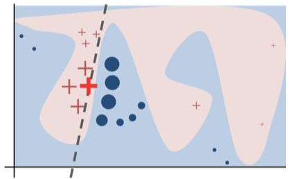
The authors of LIME have an intuitive graph as shown in Figure (E). The original complex model is represented by the blue/pink background. It is not linear. The bold red cross is the individual prediction to be explained. The algorithm of LIME does the following steps:

• Generating new samples then gets their predictions using the original model, and
• Weighing these new samples by the proximity to the instance being explained (represented in Figure (E) by size).

Then it builds a linear regression for these newly created samples including the red cross. The dashed line is the learned explanation that is locally (but not globally) faithful.

(F) How to Use LIME in Python?

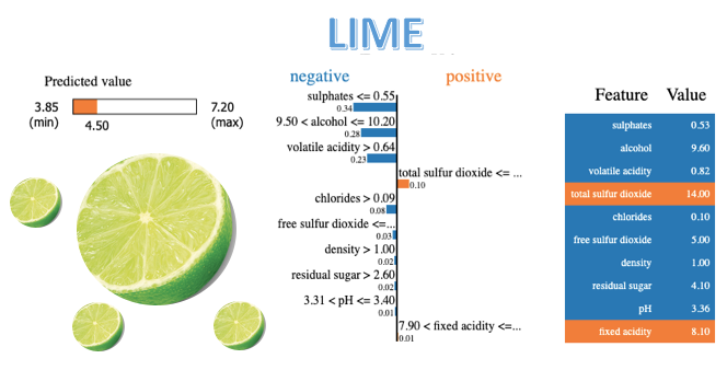
To let you compare SHAP and LIME, I use the red wine quality data used in “Explain Your Model with the SHAP Values” and “Explain Any Models with the SHAP Values — Use the KernelExplainer”. There are 1,599 wine samples. The column of the target is the quality rating from low to high (0–10). The input variables are the content of each wine sample including fixed acidity, volatile acidity, citric acid, residual sugar, chlorides, free sulfur dioxide, total sulfur dioxide, density, pH, sulphates, and alcohol. You can get the code via this Github.

The purpose of LIME is to explain a machine learning model. So I will build a random forest model in Section (F.1), then apply LIME in Section (G).

(F.1) Build a model

I am going to apply the model to the first two records of the test data X_test. The Y values of the two records are ‘6’ and ‘5’ (you can obtain them byY_test[0:2]), and the predictions are 5.58, 4.49 respectively (use model.predict(X_test[0:2])).

(F.2) Specify the LIME explainer

You will install the LIME module (pip install lime) from this Github. The code below builds the LIME model explainer.

Why is it named “lime_tabular”? LIME names it for tabular (matrix) data, in contrast to “lime_text” for text data and “lime_image” for image data. In our example all predictors are numeric. LIME perturbs the data by sampling from a Normal(0,1) and doing the inverse operation of mean-centering and scaling, according to the means and standard deviations in the training data. If you have categorical variables, LIME perturbs the data by sampling according to the training distribution and creates a binary feature of 1 if the value is the same as the instance being explained.

(G) Interpret Observation 1:

Let’s create the explanation graph for the first observation in X_test. The LIME explainer takes (i) the observation to be explained, and (ii) the model and the model prediction that needs to be interpreted. They are (i) X_test.iloc[0] and (ii) model.predict respectively. The LIME algorithm will generate new samples around X_test.iloc[0] and produce the predictions of those new samples using the model model. These steps have been described in Section (E). The code uses num_features just to specify the number of features displayed.

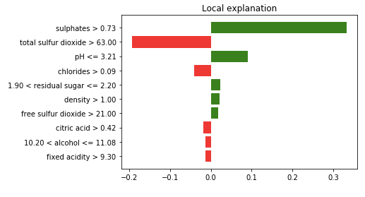
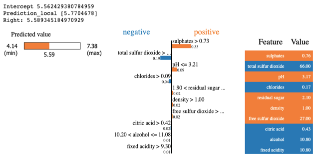
Let’s understand Figure (G.1):

• Green/Red color: features that have positive correlations with the target are shown in green, otherwise red.
• Sulphates>0.73: high sulphate values positively correlate with high wine quality.
• Total sulfur dioxide>63.0: high total sulfur dioxide values negatively correlate with high wine quality.
• ph≤3.21: low ph values positively correlate with high wine quality.
• Use the same logic to understand the rest features.

You can obtain the coefficients of the LIME model by as_list():

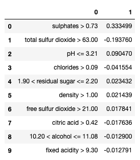
And you can show all the results in a notebook-like format:

• The LIME model intercept: 5.562,
• The LIME model prediction: “Prediction_local 5.770”, and
• The original random forest model prediction: “Right: 5.589”.

How does LIME get its Prediction_local 5.770? It is the intercept plus the sum of the coefficients. Because the intercept is 5.562 and the total of the coefficients is 0.208 (obtained by pd.DataFrame(exp.as_list())[1].sum()), the LIME prediction is 5.678 + 0.208 = 5.770.

(H) Interpret Observation 2

Let me produce the explanation graph for the second observation in X_test just to see how it works.

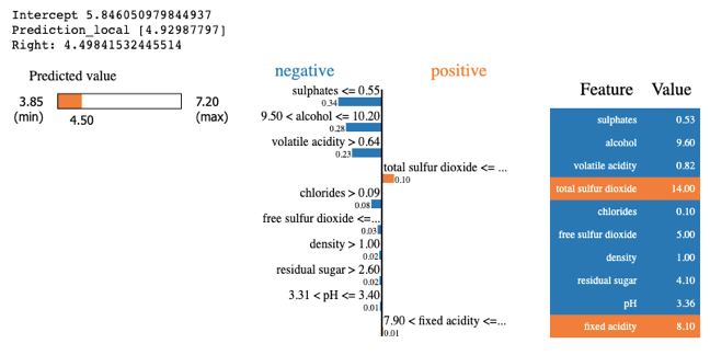
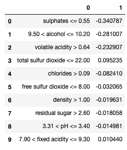
The sum of the above coefficients is -0.916. Because the intercept is 5.846, the LIME prediction becomes 5.846 -0.916 = 4.929.

The Model Explainability Article Series

For those of you who are interested in model explainability, the following sequence will be helpful:

Part I: Explain Your Model with the SHAP Values

Part II: The SHAP with More Elegant Charts

Part III: How Is the Partial Dependent Plot Calculated?

Part VI: An Explanation for eXplainable AI

Part V: Explain Any Models with the SHAP Values — Use the KernelExplainer

Part VI: The SHAP Values with H2O Models

Part VII: Explain Your Model with LIME

Part VIII: Explain Your Model with Microsoft’s InterpretML

Readers are recommended to purchase books by Chris Kuo:

• The explainable AI: https://a.co/d/cNL8Hu4
• Transfer learning for image classification: https://a.co/d/hLdCkMH
• Modern time series anomaly detection: https://a.co/d/ieIbAxM
• Handbook of Anomaly Detection: https://a.co/d/5sKS8bI