NeuralProphet (I) — Trend + Seasonality + Holidays

Many of you may have heard about the open-source Prophet module for time series forecasting. Prophet sets a paradigm in time series forecasting community. Its interpretability of the forecasts as well as interactive user-interface have been welcomed by many professionals. I covered Prophet In the series “Business Forecasting with Facebook’s Prophet”. Now, with the release of the NeuralProphet module, I am even more excited to write the tutorial series to introduce NeuralProphet to you. If you have never used Prophet before, you can click “Business Forecasting with Facebook’s Prophet”.

You may wonder what’s new in NeuralProphet, or even, what’s new in Prophet. In the tutorial series, I will start with a re-cap of Prophet and introduce NeuralProphet. Then I will add modules in a sequence. Neural Prophet inherits the trend, seasonality, holidays & events of Prophet, and expands to the auto-regressive, lagged regressors, and future regressors components. Each component can be experimented and optimized as I will show you in my tutorials.

I organize the tutorial series into digestible sizes like the following:

By following the tutorial series, you will be able to build NeuralProphet models easily and interpret your model outcomes comfortably. I incorporate the theoretical background in the context whenever it is needed. If you have built models with Prophet before, you may even consider refreshing your models with NeuralProphet which offers many compelling features.

In this first post, you will learn:

Why Prophet?
Why NeuralProphet?
Google Colab and installation of NeuralProphet
The components in NeuralProphet
Understanding the trend module
Understanding the seasonality module
The trend + seasonality modules
The trend + seasonality + holidays & events modules

Throughout the tutorials, you will see the use of out-of-time performance metrics repeatedly. This will help you to be well-grounded in the discipline of time series modeling development. The Python notebooks are available via the link in each tutorial for you to download and modify. The code for this tutorial is here.

So why wait? Let’s start.

Why Prophet?

Prophet has gained popularity for its effectiveness and interpretable forecasts. Let’s see its noticeable features. The first feature is additivity. It decomposes time series data into three main components: trend, seasonality, and holidays & events. This framework of additive components makes the model transparent and the forecasts explainable. Prophet adopts the generalized additive model (GAM) originally invented by Trevor Hastie and Robert Tibshirani in 1986. In an era of model explainability in data science, this framework makes it accessible to users with varying expertise in industry and academia. The second feature of Prophet is its automation in detecting changepoints. Changepoints are points where the time series exhibits abrupt changes in its trajectory and exist in almost any time series. The automation helps capture sudden shifts in the data and adjusts the model accordingly. You are encouraged to dig into my post “Detecting Change Points in Time Series”.

The third feature of Prophet is its flexibility in customizing changepoints, seasonality, and holidays. Users can incorporate their prior knowledge into the model, and control the model parameters for fine-tuning. The fourth feature of Prophet is uncertainty or prediction intervals for the forecast in addition to point estimates at the mean. The prediction intervals enable users to assess the risks and identify anomalies.

Why NeuralProphet?

NeuralProphet inherits the framework of Prophet and advances it with many plausible features. One noticeable enhancement is its auto-regressive (AR) module. If you come from the ARIMA (Auto-Regressive Integration Moving-Average) forecasting methods and use Prophet, you may have found a gap between the GAM framework of Prophet and the auto-regressive thinking in ARIMA. Prophet does not specify auto-regressive terms as regressors like ARIMA to model the patterns. In recent time series modeling literature, there are many works to apply neural networks to model a univariate time series. One successful work is AR-Net that use the past terms to forecast the future. NeuralProphet includes AR-net and adds it to be a new module. With the AR module, NeuralProphet reported a greater predictability over Prophet. Further, because neural networks can include hidden layers, they can capture more complex patterns that the classic ARIMA-type models. In the second tutorial, I will explain the neural networks of AR-Net and AR-module of NeuralProphet, and experiment with different neural network structures.

A time series is called a univariate time series if it uses only the information from the target variable itself to forecast the future. A time series becomes multivariate when it has other variables, called covariates, to forecast the future values of the target variable. NeuralProphet adds the lagged regressors and future regressors modules that allow for other covariates. This feature of NeuralProphet expands the univariate time series model of Prophet to a multivariate setting. Again, this will be explained in a great detail in my second tutorial.

NeuralProphet uses uncertainty estimation techniques such as quantile regression or conformal prediction, to better model the prediction intervals around the mean predicted values. Its approach to modeling seasonality is more sophisticated. It uses Fourier term seasonality at different hourly, weekly, daily, and yearly periods.

Several engineering advantages in NeuralProphet are also worth noting, especially from the perspectives of software developers. NeuralProphet is built on top of PyTorch, a popular deep-learning library. This allows software developers to scale PyTorch. NeuralProphet is designed to be extensible through its additive modules. This enables software engineers to integrate additional functionalities or customize the model according to their requirements. NeuralProphet was tested to deliver equivalent or superior quality to Prophet (Triebe et al. (2021)).

The components of NeuralProphet

Prophet’s GAM framework includes the trend, seasonality, and holidays & events as three components. NeuralProphet expands it to include the auto-regressive component, the lagged regressors and the future regressors modules, as formulated in the equation:

yˆt = T(t) + S(t) + E(t) + A(t) + L(t) + F(t)

where

T(t) = Trend at time t
S(t) = Seasonal effects at time t
E(t) = Event and holiday effects at time t
A(t) = Auto-regression effects at time t based on past observations
L(t) = Regression effects at time t for lagged observations of exogenous variables
F (t) = Regression effects at time t for future-known exogenous variables

All these modules can be individually configured and combined to compose the model. You may have found that we can turn each component turn in a sequence to build many candidate models. Then we can select a model from the model candidates.

Before we build NeuralProphet models, Let’s talk about the hardware and environment.

Using Google Colab

I recommend Google Colab as your NeuralProphet project, if you do not have GPUs on your local machine, Google Colab is a good choice. See “Start using Google Colab Free GPU” on how to set up a GPU environment for your Google Colab notebooks.

Installation of NeuralProphet

Following the standard installation pip install NeuralProphet to install NeuralProphet.

!pip install neuralprophet

If you use Google Colab, just be aware that NeuralProphet does not work with Colab unless using numpy1.23.5. You will need to uninstall numpy and install numpy1.23.5.

# neuralprophet does not work with colab unless numpy1.23.5: https://github.com/googlecolab/colabtools/issues/3752
!pip uninstall numpy
!pip install git+https://github.com/ourownstory/neural_prophet.git numpy==1.23.5

And let’s import several tools:

%matplotlib inline
from matplotlib import pyplot as plt
import pandas as pd
import numpy as np
import logging
import warnings
logging.getLogger('prophet').setLevel(logging.ERROR)
warnings.filterwarnings("ignore")

Let’s talk about the data for our modeling exercise. I used the Bike Share Daily data from Kaggle (here or here) to demonstrate the Prophet modeling in “Business Forecasting with Facebook’s Prophet”. I will continue to use it to demonstrate NeuralProphet. This dataset is a multivariate dataset that has the daily rental demand, and other weather fields like temperature or wind speed.

from google.colab import drive
drive.mount('/content/gdrive')

path = '/content/gdrive/My Drive/data/time_series'
data = pd.read_csv(path + '/bike_sharing_daily.csv')
data.tail()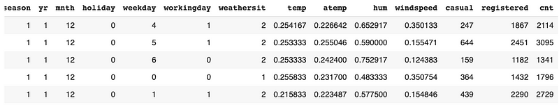

Let’s plot the bike-sharing count. We observe the demand increases in the second year, and there is a seasonal pattern.

# convert string to datetime64
data["ds"] = pd.to_datetime(data["dteday"])

# create line plot of sales data
plt.plot(data['ds'], data["cnt"])
plt.xlabel("date")
plt.ylabel("Count")
plt.show()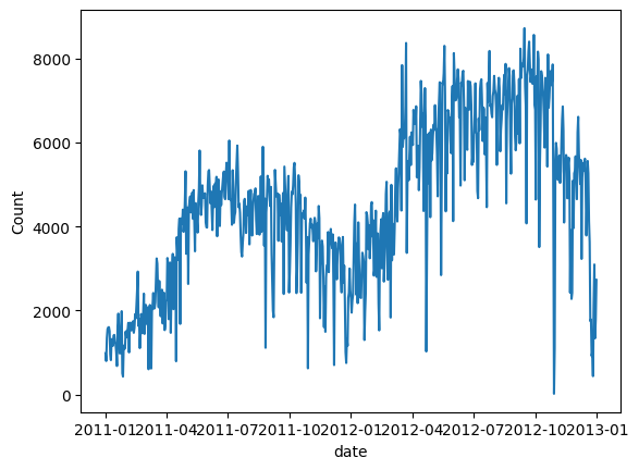

Figure (A): The bike-rental daily demand

We will do a very minimal data preparation for modeling. NeuralProphet requires the column names to be “ds” and “y” which is the same as Prophet.

df = data[['ds','cnt']]
df.columns = ['ds','y']

Let’s build a simple NeuralProphet model with all the default parameters. The goal here is to orient ourselves with its basic code and output interface. We do not provide any parameters in NeuralProphet() and we train the model using .fit().

from neuralprophet import NeuralProphet, set_log_level

# Disable logging messages unless there is an error
set_log_level("ERROR")

# Create a NeuralProphet model with default parameters
m = NeuralProphet()

# Fit the model
metrics = m.fit(df)

Once done, we will make a new data frame for the forecasts by using .make_future_dataframe(). NeuralProphet inherits this from Prophet.

# Create a new dataframe reaching 365 into the future for our forecast, n_historic_predictions also shows historic data
df_future = m.make_future_dataframe(df, 
              n_historic_predictions=True, 
              periods=365)

# Predict the future
forecast = m.predict(df_future)

# Visualize the forecast
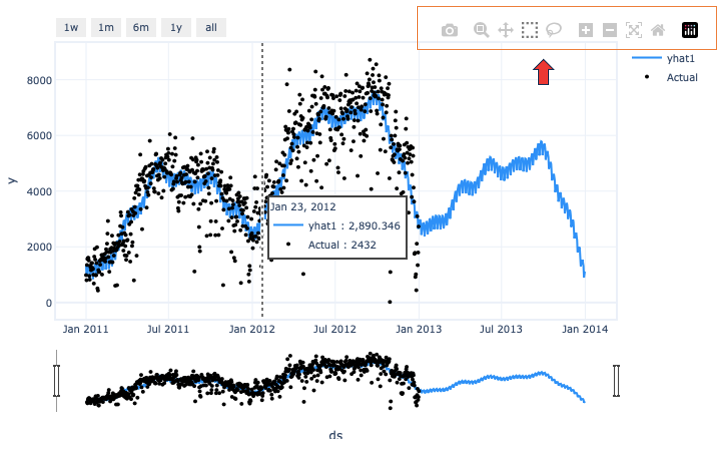
m.plot(forecast)

NeuralProphet produces interactive exhibits like the exhibit in Figure (B). The black dots are the actual data, and the blue dots and the forecasts. When you hover over a data point, it shows a box for the actual value and the forecast. It also shows a dashed vertical line to align with the time in the x-axis. This interactive exhibit is facilitated by Plotly, a popular open-source, interactive data visualization library for Python. You can zoom in and out, or download the image with the tools of Plotly in the upper right corner. If you would like to know more about Plotly, you can check “Create Beautiful Geomaps with Plotly”.

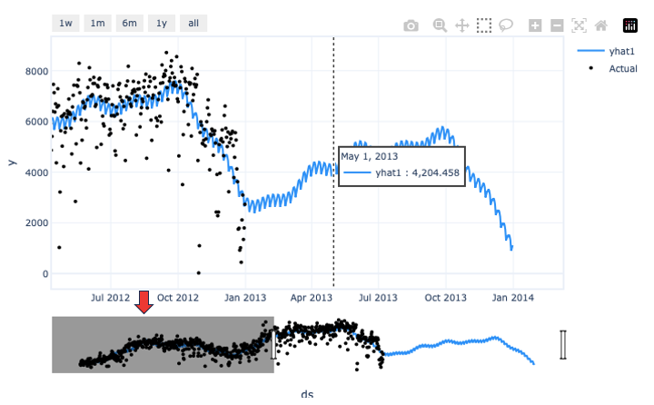
Figure (B): The main outcome of the model

At the bottom of the interactive graph is a sliding bar for you to mask unwanted data areas. I chose to mask the earlier data so I can better focus on the forecasts. Figure (C) below shows what I just did:

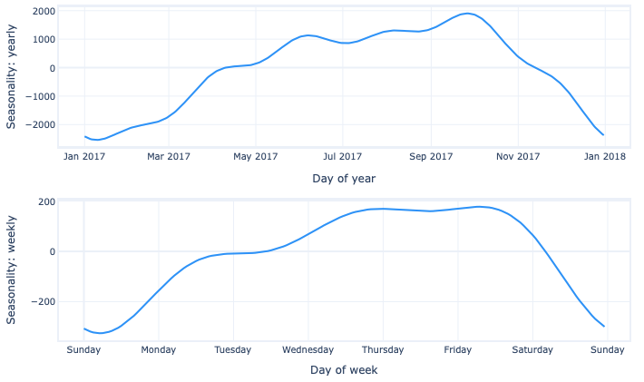
Figure (C): Using the interactive interface

NeuralProphet shows you the trend and seasonality components. See Figures (D) and (E) below. This Prophet-style interpretability helps you to engage with the users to understand the model.

m.plot_parameters(components=["trend", "seasonality"])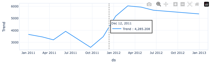

Figure (D): Interpreting the trend pattern

Figure (E): Interpreting the seasonal patterns

The trend line is not a straight line but a piecewise line. How is it produced? Let’s dig into the trend module.

Understanding the trend module

The trend of a time series is the most obvious pattern. It is a straight line over time, and the slope of the line is usually called the growth rate. However, it is quite often that time series data do not follow just one straight line. The growth rates may be different in different periods. A more intuitive trend line should be a piecewise one that looks like line segments. Prophet and NeuralProphet produce the piecewise trend to allow the growth rates to vary over time, as shown in Figure (D) above.

Let me use Figure (F) to explain the math for piecewise trend. In the scatter plot, the data patterns seem to be different before and after Year 2000. Rather than fitting all the data points with one line, we could split the data into two periods and fit two separate but connected lines. As you can see, the estimated two-piece function appears to do a much better job of describing the trend in the data. This equation is called the piecewise regression. It has a dummy variable D for the time before and after the cutting year 2000.

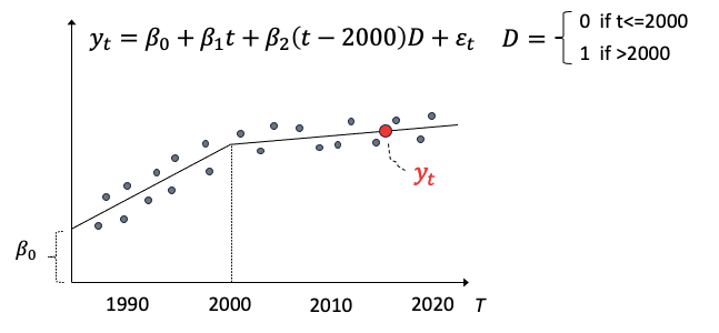
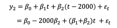
Figure (F): Using piecewise regression to model trend

Let’s formulate a piecewise trend regression. The slope for year ≤2000 is b1 and that for year > 2000 is b2. The dummy variable D is 0 if the year is before 2000 and otherwise 1. We also can rearrange the terms such that the intercepts are all together, and the slopes multiplying time:

The change point in the above example is known or pre-specified as 2000. These change points can be detected automatically. How does NeuralProphet locate the change points? Let’s find out.

The determination of the change-point locations

NeuralProphet uses a simple, semi-automatic mechanism to select the locations of the change points. It starts with n locations set apart at equal distances. This produces n-1 slopes called growth change rates to be estimated with regularization by the model. If the slopes of two connected line segments are the same or approximate, the change point is not needed and is dropped.

The last few data points of the trend segment in a time series are of more interest. If there are too many change points and trend segments in recent data, the model may over-fit especially on a small number of recent data. To mitigate this concern, NeuralProphet requires 15% of training data for the last trend segment. The forecasts therefore will not rely on just a few data points in a small trend segment. When making predictions into the unobserved future, the final growth rate is used to project linearly to the future.

Let’s do a few experiments with the trend module.

Trend module experiment 1: No change points

To observe the trend module without seasonability components, we will turn off all the seasonality components by setting them to false like the code below. Let’s assume there is no change point by setting n_changepoints=0.

# Model and prediction
m = NeuralProphet(
    # Disable change trendpoints
    n_changepoints=0,
    # Disable seasonality components
    yearly_seasonality=False,
    weekly_seasonality=False,
    daily_seasonality=False,
)
m.set_plotting_backend("matplotlib")
metrics = m.fit(df)
forecast = m.predict(df)
m.plot(forecast)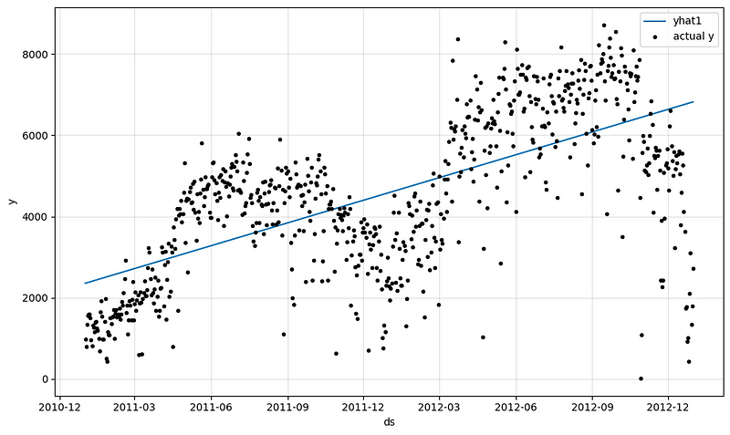

Figure (G): A naive model with no change point and no seasonality

The outcome is a simple straight line in Figure (G) or (H). Apparently, this is just an experiment.

m.plot_components(forecast, components=["trend"])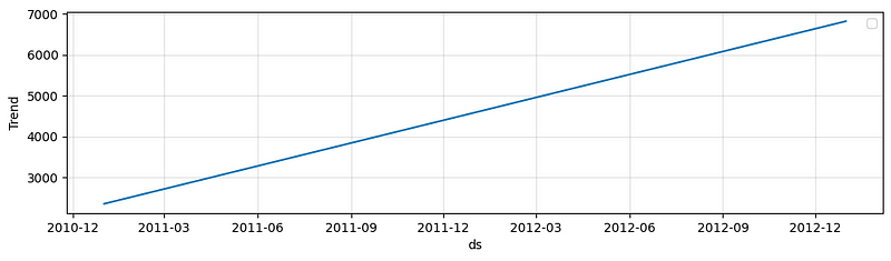

Figure (H): The trend component is a straight line in this naive model

If this naive trend line is used to project to the future, the model just extrapolate the trend linearly.

df_future = m.make_future_dataframe(df, periods=365, n_historic_predictions=True)

# Predict the future
forecast = m.predict(df_future)

# Visualize the forecast
m.plot(forecast)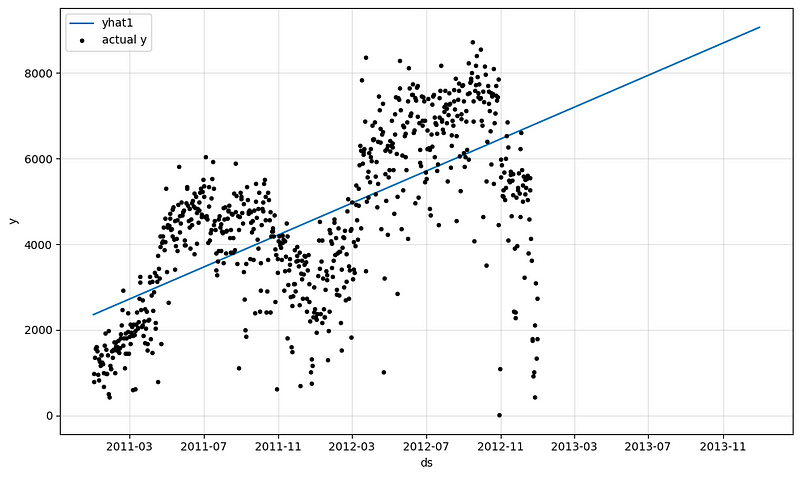

Figure (I): The forecasts of the naive model

Let’s output the performance metrics on the training set, or call the “in-time” performance metrics.

“In-time” performance metrics

Let’s print out the metrics:

metrics.tail()

The outputs are in Table (B):

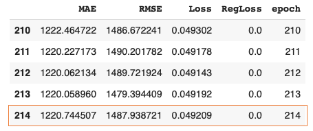
Table (B): The performance metrics for the in-time training data

The above performance metrics are on the training data. You may be asking about the performance metrics on the validation data. In time series, the validation data are the out-of-time data. Let’s see how to produce them.

“Out-of-time” performance metrics

In machine learning, we split a dataset into two parts: a training set and a testing set. The training set is used to train the model, while the testing set, representing future observations, is used to evaluate the model’s performance. When working with time series data, it is crucial to maintain the temporal order of observations. This is because time series models rely on the assumption that past observations are informative about future observations. We split the dataset into “in-time” and “out-of-time”. “Out of time” data in time series analysis are used to evaluate the model predictability for the data that the model has not seen.

Below we will use the utility function .split_df() of NeuralProphet to split into “in-time” and “out-of-time”. Conventionally, we use 20% of the data for validation, which means the last 20% data are reserved as the out-of-time data.

# Model and prediction
m = NeuralProphet(
    # Disable change trendpoints
    n_changepoints=0,
    # Disable seasonality components
    yearly_seasonality=False,
    weekly_seasonality=False,
    daily_seasonality=False,
)
df_train, df_test = m.split_df(df, valid_p=0.2)
metrics = m.fit(df_train, validation_df=df_test, progress="bar")
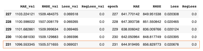
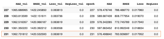
metrics.tail()

The outputs are:

Table (C): The performance metrics for the out-of-time validation data

The MAE and RMSE in Table (C) are the results of the training set. They are close to those in Table (B). The MAE_val and RMSE_val are the performance on the validation set. Do not be surprised that they are much higher than the results of the training set. Later, we will experiment with different parameter settings and we will use the out-of-time performance metrics as well.

Now let’s allow NeuralProphet to search for the change points in the 2nd experiment.

Trend module experiment 2: automatic change point detection

We still disable all the seasonality components and this time comment out n_changepoints=0 to let NeuralProphet search for the change points.

# Model and prediction
m = NeuralProphet(
    # Use the default number of change trend points (10)
    # n_changepoints=0,
    # Disable seasonality components
    yearly_seasonality=False,
    weekly_seasonality=False,
    daily_seasonality=False,
)
m.set_plotting_backend("matplotlib")  # Use matplotlib due to #1235
metrics = m.fit(df)
forecast = m.predict(df)
m.plot(forecast)

The outcome is a piecewise trend line in Figure (J).

Figure (J): The model with change points

To save space, here we only show the performance metrics of the training set:

metrics.tail()

The outputs are:

Table (D): The performance metrics for the in-time training data of the model with change points

If you compare the MAE and RMSE in Table (D) to those in Table (B), you will find they are smaller. This is because we allow for change points and the model fits better.

Change point detection is an important topic. The article “Detecting the change points in a time series” details the change point detection algorithms, and this book includes the change point detection algorithms in the Appendix.

Having learned the trend module, let’s move on to the seasonality module.

Understanding the seasonality module

Seasonality is the recurring patterns over fixed time intervals, such as daily, weekly, or yearly cycles. Let’s still turn off the change point detection so we can observe the seasonality patterns. Now let’s turn on the seasonability components by setting the weekly and yearly patterns to True. This daily time series has no hourly pattern so we do not need daily_seasonality.

# Model and prediction
m = NeuralProphet(
    # Disable trend changepoints
    n_changepoints=0,
    # Enable all seasonality components
    yearly_seasonality=True,
    weekly_seasonality=True,
    daily_seasonality=False,
)
df_train, df_test = m.split_df(df, valid_p=0.2)
metrics = m.fit(df_train, validation_df=df_test, progress="bar")

forecast = m.predict(df)
m.plot(forecast)

The outcome with seasonality components and trend without change points becomes this:

Figure (K): The model with seasonality but no change point

Let’s explain the seasonality component with the following code.

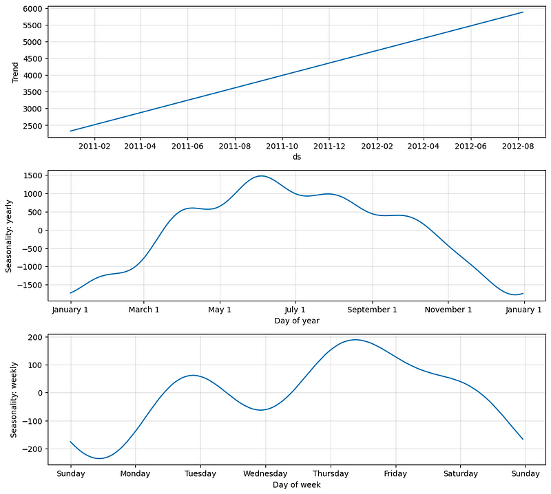
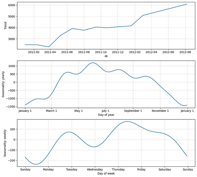
m.plot_parameters(components=["trend", "seasonality"])

The outcome is in Figure (L). The first graph shows the monthly variation in a year. There is a high demand in summer and a low demand in winter. The second graph shows the variation in a week in that the demand for bike rides is high on weekdays and low on weekends.

Figure (L): The components of the model with seasonality but no change point

Let’s see the performance metrics of the training and test datasets.

metrics.tail()

The outputs are:

Table (E): The performance metrics of the model with seasonality but no change point

What is the mathematical formula to model seasonality? The peaks or valleys in seasonality look like a collection of sine and cosine functions with varying heights. Such periodic patterns in time series can be modeled brilliantly by the Fourier terms (Harvey & Shephard, 1993). The Fourier series is a mathematical tool that represents a periodic function as the sum of sine and cosine waves with different frequencies and amplitudes. Both Prophet and NeuralProphet use Fourier terms to model seasonality (Taylor & Letham, 2017). The following equation defines Fourier terms.

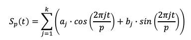
k refers to the number of Fourier terms for the periodicity p like daily data (p = 365.25) or weekly data (p = 52.18). A case of k=2 and p=52.18 means the weekly data will be modeled by two sets of cosine and sine values with coefficients a1, b1, a2, and b2 respectively. The result will be a smooth curve for the weekly pattern. If k is high, the Fourier terms have a high level of flexibility to fit complex season patterns. But that also means the risks of overfitting. The k values have to be chosen for general purposes. Prophet and NeuralProphet set the default k values. The default number of Fourier terms per seasonality are:

k = 6 for p = 365.25 yearly,
k = 3 for p = 7 weekly, and
k = 6 for p = 1 daily seasonality.

If the data is of daily frequency, the model will enable yearly seasonality if the data spans two years or more. Weekly patterns will be added if two or more weeks of data are available.

Knowing the seasonality module, let’s build a model with trend and seasonality.

Trend + Seasonality

We are ready to put together the trend and seasonality modules.

# Model and prediction
m = NeuralProphet(
    #n_changepoints=10,
    yearly_seasonality=True,
    weekly_seasonality=True,
    daily_seasonality=False,
)
m.set_plotting_backend("matplotlib")  # Use matplotlib

df_train, df_test = m.split_df(df, valid_p=0.2)
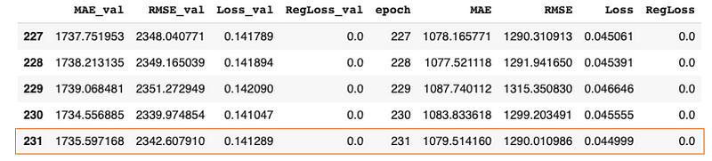
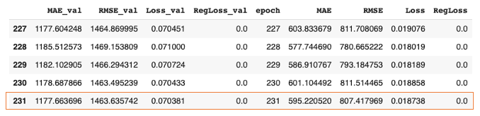
metrics = m.fit(df_train, validation_df=df_test, progress="bar")
metrics.tail()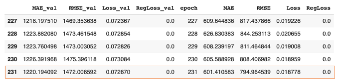

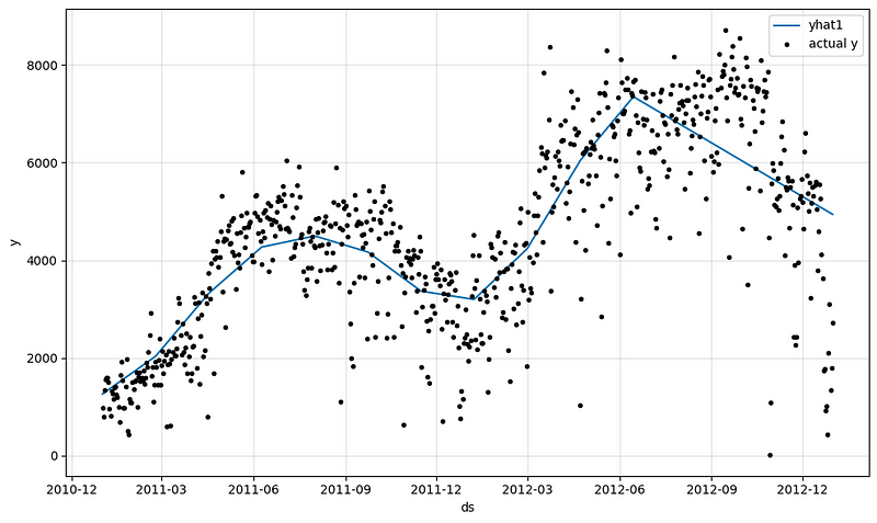
Table (F): The performance metrics of the model with change points and seasonality

Let’s plot the trend and seasonality components:

m.plot_parameters(components=["trend", "seasonality"])

The outputs are:

Figure (I): The components of the model with change points and seasonality

Now we are ready to add the holidays & events to our model.

Trend + Seasonality + Holidays & Events

NeuralProphet lets you add country holidays just like Prophet. The trend + seasonality + holidays model can provide the basic model for most business times series. NeuralProphet adopts the definitions for the holidays and events in the open-source python-holidays module. Because our bike-ride data is in the United States, I use the United States holidays & events for the country holidays.

# Model and prediction
m = NeuralProphet(
    #n_changepoints=10,
    yearly_seasonality=True,
    weekly_seasonality=True,
    daily_seasonality=True,
)
m = m.add_country_holidays("US")

m.set_plotting_backend("matplotlib")  # Use matplotlib

df_train, df_test = m.split_df(df, valid_p=0.2)
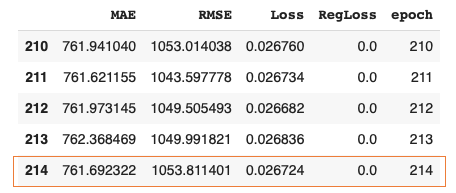
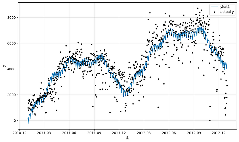
metrics = m.fit(df_train, validation_df=df_test, progress="bar")
metrics.tail()

The outputs are:

Table (G): The performance metrics of the model with trend, seasonality, and holidays

It is straightforward. Let’s see how to add custom events.

Custom events

NeuralProphet lets you specify custom events just like Prophet. You will add the events using add_events() and mark on the dataset using create_df_with_events(). For our bike-ride data, I suppose there were three known promotional events by the largest retailer in the city.

df_events = pd.DataFrame(
    {
        "event": "special_events",
        "ds": pd.to_datetime(
            [
                "2018-11-23",
                "2018-11-17",
                "2018-04-11",
            ]
        ),
    }
)

# Model and prediction
m = NeuralProphet(
    #n_changepoints=10,
    yearly_seasonality=True,
    weekly_seasonality=True,
    daily_seasonality=False
)
m = m.add_country_holidays("US")

m.add_events("special_events")

df_all = m.create_df_with_events(df, df_events)

m.set_plotting_backend("matplotlib")  # Use matplotlib

df_train, df_test = m.split_df(df_all, valid_p=0.2)
metrics = m.fit(df_train, validation_df=df_test, progress="bar")
metrics.tail()

The performance metrics are:

Table (H): The performance metrics of the model with trend, seasonality, and holidays and custom events

I guess we need to take a class break, don’t we?

Conclusions

In this post, we learned the additivity of the NeuralProphet model. We learned the piecewise model in the trend module and experimented with change point detection. We added seasonality and holidays to the trend step-by-step. We have also shown the “in-time” and “out-of-time” performance metrics in several experiments.

In the next post, we will learn how classical auto-regressive thinking is built in the AR module through neural networks. This is the main reason why NeuralProphet adds the prefix “Neural” to Prophet. The neural network approach is also applied to other variables and the model becomes a multivariate model. We will expand the univariate model in this post to a multivariate model to increase predictability. Let’s continue!

References

Oskar Triebe, Hansika Hewamalage, Polina Pilyugina, Nikolay Laptev, Christoph Bergmeir, & Ram Rajagopal. (2021). NeuralProphet: Explainable Forecasting at Scale.
Harvey, Andrew C, and Neil Shephard. 1993. “Structural time series models.” Handbook of Statistics, (edited by G.S. Maddala, C.R. Rao and H.D. Vinod), Vol. 11:Econometrics: 261–302. Amsterdam: North Holland.